Estimation, Prediction, Hypothesis Tests
import pandas as pd
import numpy as np
from scipy import stats
import matplotlib.pyplot as plt
import seaborn as sns
import preliz as pz
from tqdm.auto import tqdm
import pymc as pm
plt.rcParams["figure.figsize"] = (15,3)
plt.style.use('ggplot')
np.random.seed(1337) # for consistency
Exercise 1: Maternity Ward Planning
The maternity ward of a small regional hospital decided to use Bayesian statistics to better plan the expected daily number of beds needed. In particular, it should also be assessed whether a total number of 20 beds will with a few exceptions be enough. They have measured the following data for 30 nights and already want to start their analysis, even before more data are collected:
beds = np.array([ 6, 11, 12, 9, 11, 10, 9, 18, 9, 18, 12, 14, 9, 11, 10, 15, 13, 11, 14, 12, 11, 8, 11, 13, 11, 12, 20, 5, 13, 16])a) Check Poisson distribution assumptions
For a start, they think it is good to work with a Poisson distribution as likelihood. Verify quickly that this idea is not totally wrong by checking whether the assumptions of the Poisson distribution are (more or less) fulfilled.
np.mean( beds )np.float64(11.8)np.var( beds )np.float64(10.76)Variance and mean are (more or less) similar, let’s proceed with a Poisson distribution.
b) Elicit a prior
First you have to elicit a prior distribution for . For convenience, you use a Gamma distribution. The nurses tell you that they guess around 15 beds are occupied on average per night, a few times it can only be 10 beds and the number 20 beds is only very rarely exceeded. Choose an appropriate Gamma prior that reflects this experience.
Experiment until approximately variance from exercise description is reached:
r = 2.5
s = 15 * r
pz.Gamma(s, r).plot_pdf()
<Axes: >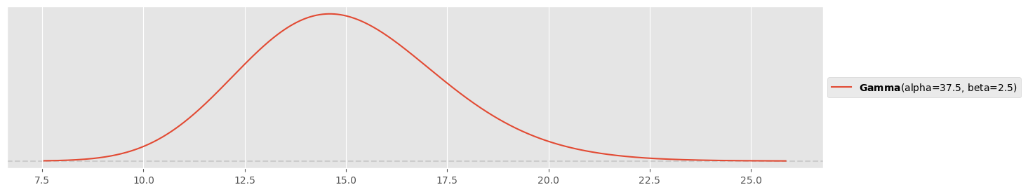
r, s(2.5, 37.5)c) Sample from prior
You’re a bit unsure whether you have used the correct parameters for the Gamma distribution (confusion between , and and ). For this reason you decide to sample only from your prior first and look at the resulting distribution of samples. Do this with PyMC, add only
lbd = pm.Gamma('lbd', alpha=s, beta=r)and then use pm.sample() to simulate samples from the prior. Produce a density plot (e.g. with pm.plot_posterior() or pm.plot_trace()) and verify that it looks the same as the prior you have elicited in the previous part.
with pm.Model() as maternity_ward_model:
    lbd = pm.Gamma( 'lbd', alpha=s, beta=r )
trace = pm.sample( 1000 )pm.plot_trace( trace );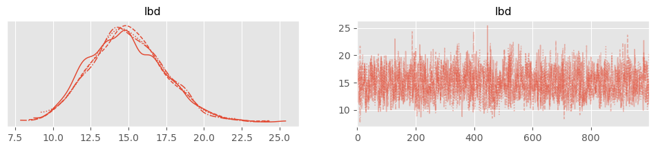
Looks as defined!
d) Sample from posterior
Use an MCMC simulation with PyMC to produce 4000 samples from the posterior and verify that your simulation is nominal by applying the usual diagnostic tools (trace/rank plot, density plot, autocorrelation plot, , ESS).
with pm.Model() as maternity_ward_model:
    lbd = pm.Gamma( 'lbd', alpha=s, beta=r )
    y = pm.Poisson( 'y', mu=lbd, observed=beds )
trace = pm.sample( 1000 )Trace and density plot:
pm.plot_trace( trace, kind="rank_bars" )array([[<Axes: title={'center': 'lbd'}>,
<Axes: title={'center': 'lbd'}, xlabel='Rank (all chains)', ylabel='Chain'>]],
dtype=object)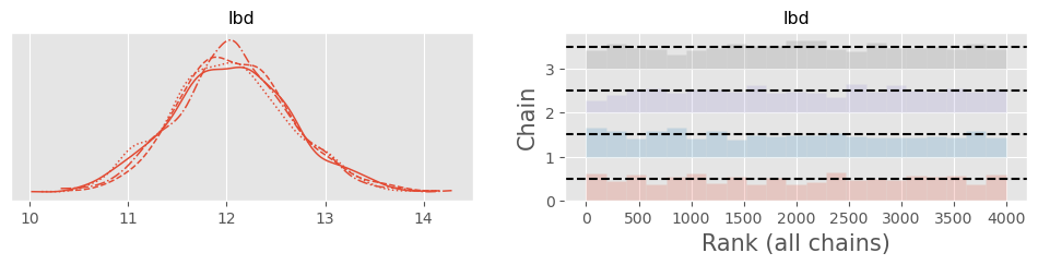
Autocorrelation plot:
pm.plot_autocorr( trace, combined=True );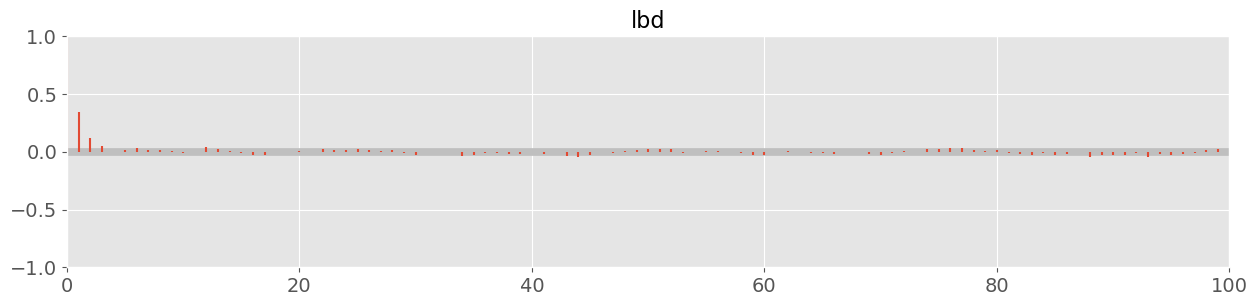
pm.rhat( trace )pm.ess( trace )Looks nominal!
e) Plot HDI
Plot the posterior density for with pm.plot_posterior() and make sure that it displays a 95% highest density interval. What are the posterior mean and standard deviation? Formulate how you would tell your result to the supervisor of the maternity ward.
pm.plot_posterior( trace, hdi_prob=0.95 )<Axes: title={'center': 'lbd'}>
pm.summary( trace, hdi_prob=0.95 )“After considering the 30 measurements, I believe to 95% that the mean number of beds used per night is somewhere between 10.9 and 13.2, if I had to guess a number, I would say 12. The standard deviation is quite small with ±0.6 beds. However the mean only reflects my model knowledge, but not my predictions!”
f) Predict exceeding of beds
The supervisor wants to know your prediction for the expected number of days per year when the total number 20 beds is exceeded. What do you tell them?
Hint: Compute the posterior predictive distribution first as done in the lecture (see accompanying notebooks) with pm.sample_posterior_predictive().
with maternity_ward_model:
    y_new = pm.Poisson('y_new', mu=lbd)
predictions = pm.sample_posterior_predictive(trace, var_names=["y_new"])365 * np.mean( predictions.posterior_predictive.y_new > 20 ).valuesnp.float64(4.65375)Around 4-5 days per year!
g) Would more data help?
Will your model get much better with more data? Compute the proportion of aleatoric and epistemic uncertainty with respect to the total predictive uncertainty.
Hint: Apply the formulas from the lecture and use that for a Poisson distribution .
aleatoric_var = np.mean( trace.posterior.lbd.values )
epistemic_var = np.var( trace.posterior.lbd.values )
pred_var = np.var( predictions.posterior_predictive.y_new.values )
np.round( np.array( [aleatoric_var, epistemic_var] ) / (aleatoric_var+epistemic_var) * 100, 1 )
array([97.1, 2.9])Aleatoric variance makes up 97%. More data will not yield much improvement here!
Exercise 2: Toilet paper A/B testing
A large tech company wants to reduce the amount of toilet paper used in their facilities, first of all to save some money but of course also to advertise their efforts for sustainability. To this end, they replace the original toilet paper rolls with rolls with thinner paper. However, a fear of the facility management is that people will just use more toilet paper to compensate for the thinner rolls. To this end, they plan to conduct a very preliminary study (this is where you come into play).
Before the rolls are replaced with the new ones, the total use in kilograms is measured each week for 5 weeks (‘b’ for before):
After the replacements, another 5 weekly measurements of total weight in kilograms are taken (‘a’ for after):
y_b_obs = np.array([181, 152, 148, 146, 171])
y_a_obs = np.array([163, 153, 146, 126, 142])
a) Create the Model
Assume the same normally distributed model as used in the practical railway counter queue example in the lecture and simulate samples from the posterior distribution to get a posterior understanding of the values for , , and . Instead of eliciting a prior, use the empirical Bayes approach and set the priors:
where is the mean value of and its variance (careful, use ddof=1 in Numpy—why?). Note that by choosing the variance of the prior on as large as the standard deviation of the data we create very weak priors.
with pm.Model() as toilet_paper_model:
    μ_b = pm.Normal( 'μ_b', mu=np.mean(y_b_obs), sigma=np.std(y_b_obs, ddof=1) )
    μ_a = pm.Normal( 'μ_a', mu=np.mean(y_a_obs), sigma=np.std(y_a_obs, ddof=1) )
    σ_b = pm.Exponential( 'σ_b', lam=1/np.std(y_b_obs, ddof=1) )
    σ_a = pm.Exponential( 'σ_a', lam=1/np.std(y_a_obs, ddof=1) )
    y_b = pm.Normal( 'y_b', mu=μ_b, sigma=σ_b, observed=y_b_obs )
    y_a = pm.Normal( 'y_a', mu=μ_a, sigma=σ_a, observed=y_a_obs )
trace = pm.sample( 1000 )Check chain quickly:
pm.plot_trace( trace )
plt.tight_layout()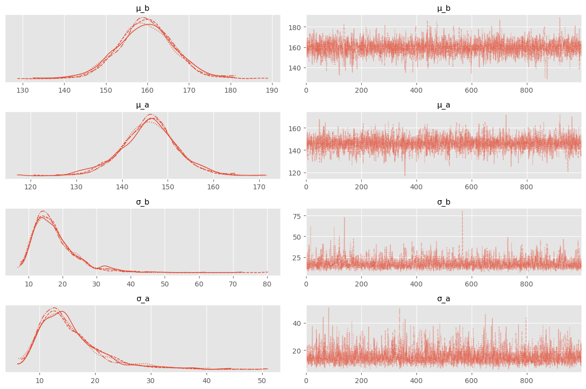
Looks good!
b) Plot the HDI
What is a 80% HDI for the saved relative total toilet paper weight ? Would you recommend to continue to use the new toilet paper?
reldiff = (trace.posterior.μ_b - trace.posterior.μ_a) / trace.posterior.μ_b
pm.plot_posterior( reldiff, hdi_prob=0.8 )
<Axes: title={'center': 'x'}>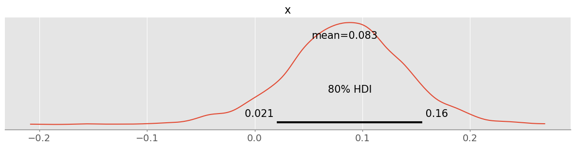
pm.hdi( reldiff, hdi_prob=0.8 ).x.valuesarray([0.02062758, 0.15572381])With a plausibility of 80%, about 1-15% toilet paper mass less is used! This does not appear very certain and more data will be needed for a better number. However it is already now quite clear that likely the weekly mass of toilet paper used was reduced.
c) Compute the odds of the experiment
The facility head promised before the experiment: “I am very sure that we will cut down the amount of toilet paper (in kg) at least by 20%!” Verify his statement in the form of a hypothesis test and compute the odds that his statement is true. Did he exaggerate or not?
: %
: %
PH1d = np.mean( reldiff.values >= 0.2 )
PH1dnp.float64(0.0165)PH2d = 1-PH1d
PH2dnp.float64(0.9835)posterior_odds = PH1d / PH2d
posterior_oddsnp.float64(0.01677681748856126)Given the measured data, the odds for his hypothesis are very small!
d) Quantify the plausibility of statement
After you destroyed his illusions, he says: “Ok, but the data shows that it’s at least 10%!” Quantify the plausibility of this statement.
np.mean( reldiff.values >= 0.1 )np.float64(0.38175)This hypothesis is true with a probability of 38% (number might change slightly in multiple runs)! The value might as well be smaller!
Exercise 3: Defective Screws
A company produces a novel type of medical implant screws. The production machines have recently been set up by the engineering team and are at a steady production of 1000 screws per day. Very rarely, the machines produce a defective screw that does not fullfil the rigorous requirements for medical devices and has to be thrown away. So far, after 30 days of production, this has occured 5 times.
a) Estimate the defect rate
You are tasked to estimate the defect rate of the new machines. Choose a prior that follows an exponential distribution (instead of the beta distribution that we used so far for binomial problems). Your prior distribution should reflect the measured rate of 5 in 30’000 as a mean rate (as allowed in empirical Bayes). Visualize your prior.
Prior:
mean_rate = 5/30000
pz.Exponential(lam=1/mean_rate).plot_pdf()
<Axes: >
b) Estimate the posterior distribution
Given this prior and the data, estimate and visualize a posterior distribution for the rate of defective screws. What is the 90% HDI of your estimate of ?
Run simulation:
with pm.Model() as defective_screw_model:
    pi = pm.Exponential( 'pi', lam=1/mean_rate)
    y = pm.Binomial( 'y', n=30000, p=pi, observed=5 )
trace = pm.sample( 1000 )Diagnostics:
pm.plot_trace( trace )array([[<Axes: title={'center': 'pi'}>, <Axes: title={'center': 'pi'}>]],
dtype=object)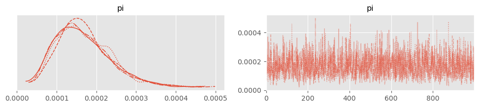
pm.plot_autocorr( trace, combined=True )<Axes: title={'center': 'pi'}>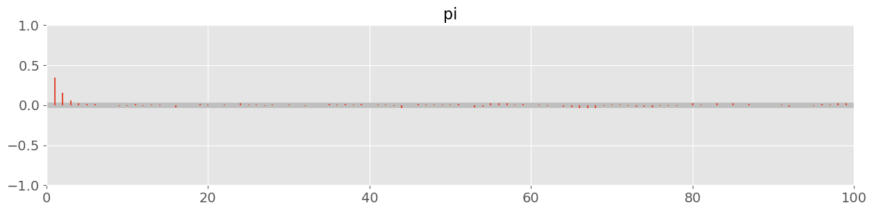
Looks good!
Visualize posterior:
pm.plot_posterior( trace, hdi_prob=0.9 )<Axes: title={'center': 'pi'}>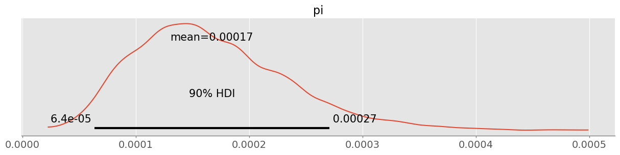
pm.hdi( trace, hdi_prob=0.9 ).pi.valuesarray([6.35819267e-05, 2.70882057e-04])90% HDI is between 6 in 100’000 and 2.7 in 1000. There is still quite some uncertainty!
c) Predict defective screws
What number of defective screws can you expect for the next 30 days? (for better planning sales require a 90% HDI) What are the proportions of aleatoric and epistemic uncertainty in the total predictive uncertainty? Can you make promises to the sales departement that you will be much better next time when you have more data?
with defective_screw_model:
    y_new = pm.Binomial('y_new', n=30000, p=pi)
predictions = pm.sample_posterior_predictive(trace, var_names=["y_new"])pm.plot_posterior( predictions.posterior_predictive.y_new, hdi_prob=0.9 )<Axes: title={'center': 'y_new'}>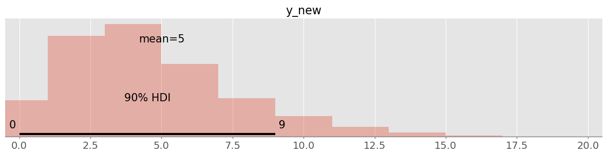
pm.hdi( predictions.posterior_predictive.y_new, hdi_prob=0.9 ).y_new.valuesarray([0., 9.])Within the next 30 days, I believe to 90% that between 0-9 screws will be defective.
Aleatoric and epistemic uncertainty:
n_new = 30000
aleatoric_vars = n_new * trace.posterior.pi.values * (1-trace.posterior.pi.values)
aleatoric_var = np.mean( aleatoric_vars )
aleatoric_varnp.float64(5.008670453974596)epistemic_var = np.var( trace.posterior.pi.values * n_new )
epistemic_varnp.float64(4.129590835900785)Looks like there is the same amount of epistemic variance and aleatoric variance - more data should improve the predictions.
Check: Real predictive uncertainty vs theoretical one:
predictive_var = np.var( predictions.posterior_predictive.y_new.values )
predictive_var, aleatoric_var+epistemic_var
(np.float64(9.131204437500001), np.float64(9.13826128987538))d) Update your estimate
After the next 30 days you get an update from the engineering team: After total 60 days (previous period and this period), 60’000 screws have been produced whereas 8 have been found to be defective. Update your estimate in c) and recompute the proportions of aleatoric and epistemic uncertainty. You may keep your previous prior and add the whole data (, ) to it.
Re-run simulation with more data:
with pm.Model() as defective_screw_model2:
    pi = pm.Exponential( 'pi', lam=1/mean_rate)
    y = pm.Binomial( 'y', n=60000, p=pi, observed=8 )
trace2 = pm.sample( 1000 )Visualize posterior belief for proportion :
pm.plot_posterior( trace2, hdi_prob=0.9 )<Axes: title={'center': 'pi'}>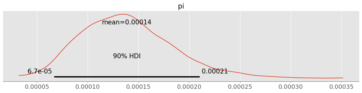
pm.hdi( trace2, hdi_prob=0.9 ).pi.valuesarray([6.22845358e-05, 2.04071282e-04])90% HDI changed to between 7 in 10000 and 2 in 1000. In particular the upper bound is considerably lower.
Prediction for the next 30 days:
with defective_screw_model2:
    y_new = pm.Binomial('y_new', n=30000, p=pi)
predictions2 = pm.sample_posterior_predictive(trace2, var_names=["y_new"])pm.plot_posterior( predictions2.posterior_predictive.y_new, hdi_prob=0.9 )<Axes: title={'center': 'y_new'}>
pm.hdi( predictions2.posterior_predictive.y_new, hdi_prob=0.9 ).y_new.valuesarray([0., 7.])Within the next 30 days, I believe to 90% that between 0-7 screws will be defective. There is still considerable uncertainty.
Aleatoric and epistemic uncertainty for 30 days prediction:
n_new = 30000
aleatoric_vars = n_new * trace2.posterior.pi.values * (1-trace2.posterior.pi.values)
aleatoric_var = np.mean( aleatoric_vars )
aleatoric_varnp.float64(4.15177581882005)epistemic_var = np.var( trace2.posterior.pi.values * n_new )
epistemic_varnp.float64(1.8507032509875625)Proportions:
np.array([aleatoric_var, epistemic_var]) / (aleatoric_var+epistemic_var)array([0.69167685, 0.30832315])Check:
predictive_var = np.var( predictions2.posterior_predictive.y_new.values )
predictive_var, aleatoric_var+epistemic_var
(np.float64(5.8460699375), np.float64(6.002479069807612))Note: Because the predicted numbers and the involved uncertainties are low and of about the same magnitude, comparing aleatoric and epistemic uncertainty can also be misleading here. You can play around with this by e.g. assuming that 12 screws of 60’000 were defective instead of 8.
Exercise 4: Baby Diapers
So far you have used Pampers diapers for your baby. Within two weeks, you have used 81 diapers in total and have experienced 4 leaks where the diapers did not hold anymore, resulting in a total mess. After speaking to a friend, he recommends using Lidl’s own diaper brand that costs around as half as Pampers diapers. You are eager to try them!
After one week, you have used 39 diapers in total and have already experienced 3 leaks! You are annoyed. Is it reasonable to stop the experiment and to abandon the Lidl diapers?
Give your answer with a Bayesian hypothesis test using a binomial likelihood and a flat prior for simplicity.
Hint: Check the posterior distribution of the rate difference Lidl - Pampers.
Build the model:
with pm.Model() as diapers_model:
    leak_rate_pampers = pm.Beta( 'leak_rate_pampers', alpha=1, beta=1 )
    leak_rate_lidl = pm.Beta( 'leak_rate_lidl', alpha=1, beta=1 )
    y_pampers = pm.Binomial( 'y_pampers', p=leak_rate_pampers, n=81, observed=4 )
    y_lidl = pm.Binomial( 'y_lidl', p=leak_rate_lidl, n=39, observed=3 )
trace = pm.sample( 1000 )pm.plot_trace( trace )
plt.tight_layout()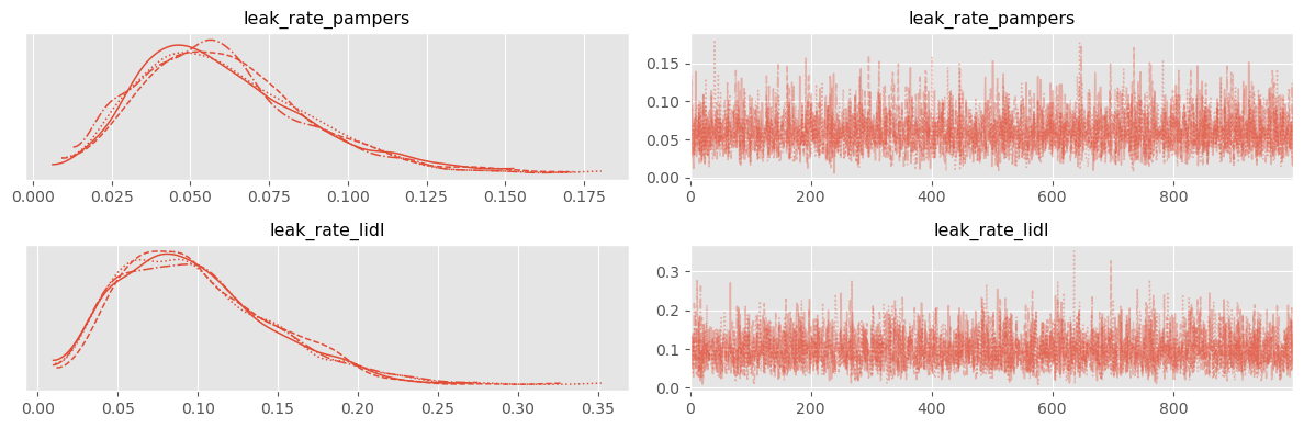
pm.summary( trace )Obviously we estimate the “mean leak rate” higher for the Lidl brand. But can we really say that they are worse?
diff = trace.posterior.leak_rate_lidl - trace.posterior.leak_rate_pampers
pm.plot_posterior( diff, hdi_prob=0.8 )
<Axes: title={'center': 'x'}>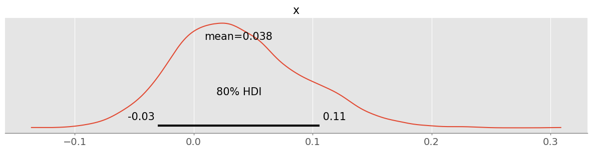
The resulting HDI of the difference includes 0 at the 80% level and consequently is not significant at the 80% level. It will definitely not be significant at the 90% or 95% level. The data does not indicate that we should already stop our experiment, rather we should collect more “data” 💩