Exercises Continous Problems and Conjugate Families

import pandas as pd
import numpy as np
from scipy import stats
import matplotlib.pyplot as plt
import seaborn as sns
import preliz as pz
from tqdm.auto import tqdm
plt.rcParams["figure.figsize"] = (15,3)

Exercise 1: Prior elicitation¶

(this is the slightly adapted exercise 3.1 from Bayes rules!)

In each situation below, tune a $Beta(\alpha,\beta)$ model that accurately reflects the given prior information and visualize it. In many cases, there’s no single “right” answer, but rather multiple “reasonable” answers.

Hint: Often you can constrain the possible values for $\alpha$ and $\beta$ using a given expectation or variance:

E[\pi]=\frac{\alpha}{\alpha+\beta}

(1)

Var[\pi]=\frac{\alpha\beta}{(\alpha+\beta)^{2}(\alpha+\beta+1)}

(2)

This might save you time when trying out different values for $\alpha$ and $\beta$ . If you’re not in the mood for calculations however, just try them out!

a) Your friend applied to a job and tells you: “I think I have a 40% chance of getting the job, but I’m pretty unsure.” When pressed further, they put their chances between 20% and 60%.

E[\pi] = 0.4 = \frac{\alpha}{\alpha+\beta} \quad \Rightarrow \frac{\alpha}{\beta} = \frac{E[\pi]}{1-E[\pi]} = \frac23

(3)

Try out different values given the constraint above:

beta = 15
alpha = 2/3 * beta
pz.Beta(alpha, beta).plot_pdf()
print( "alpha = {}, beta = {}".format( alpha, beta ) )

alpha = 10.0, beta = 15

However Beta(6,9) or Beta(12,18) could also be reasonable!

b) A scientist has created a new test for a rare disease. They expect that the test is accurate 80% of the time with a variance of 0.005.

$\displaystyle{\frac{\alpha}{\beta} = \frac{E[\pi]}{1-E[\pi]} = 0.8/0.2 = 4} \quad \Rightarrow \alpha = 4\beta$

$\text{Var}[\pi] = \displaystyle{\frac{\alpha\beta}{(\alpha+\beta)^2 (\alpha + \beta + 1)} = \frac{4\beta^2}{(5\beta)^2 \; (5\beta + 1)} = \frac{4}{25 \; (5\beta + 1)} = 0.005} \; \Rightarrow 5\beta + 1 = \frac{4}{25 \cdot 0.005} \; \Rightarrow \beta = \frac15 \left(\frac{4}{25 \cdot 0.005}-1\right) = 6.2$

beta = 1/5 * (4/(25*0.005)-1)
beta

6.2

alpha = 4*beta
alpha

24.8

pz.Beta(alpha, beta).plot_pdf()

<Axes: >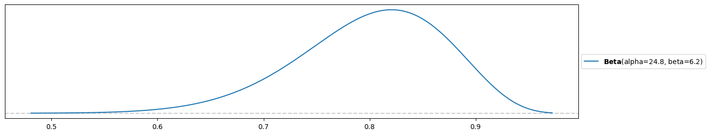

c) Another scientist in the same field claims that he expects the same accuracy, however a ten times larger variance of 0.05. Can the beta distribution model this prior expectation well?

Using the same formula:

beta = 1/5 * (4/(25*0.05)-1)
beta

0.44000000000000006

alpha = 4*beta
alpha

1.7600000000000002

pz.Beta(alpha, beta).plot_pdf()

<Axes: >

pz.Beta(alpha, beta).mean(), pz.Beta(alpha, beta).var()

(0.8, 0.05)

Oops! This beta distribution has the correct expectation and variance, but does not model what we want. We would rather have a distribution centered around 0.8. This is the price of reducing all possible prior to a two-dimensional family (parameterized by $\alpha$ and $\beta$ ). An alternative might be a truncated normal distribution:

pz.TruncatedNormal(mu=0.8, sigma=np.sqrt(0.05), lower=0, upper=1).plot_pdf()

<Axes: >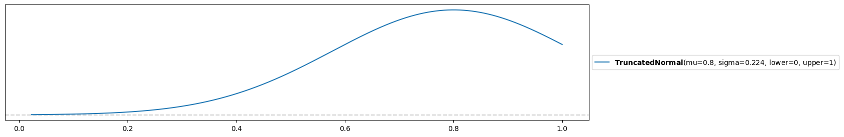

However it’s hard to say whether this is what we want and depends on the application. You might try with more bounded distributions that are listed here.

d) Your Aunt Jo is a successful mushroom hunter. She boasts: “I expect to find enough mushrooms to feed myself and my co-workers at the auto-repair shop 90% of the time, but if I had to give you a likely range it would be between 85% and 100% of the time.”

Ratio through expectation:

$\frac{\alpha}{\beta} = \frac{E[\pi]}{1-E[\pi]} = \frac{0.9}{0.1} = 9$ .

Tuning by hand, trying until the range is more or less correct:

beta = 5 # tried 1, 2, 3, 4, 5
alpha = 10*beta
pz.Beta( alpha, beta ).plot_pdf()

<Axes: >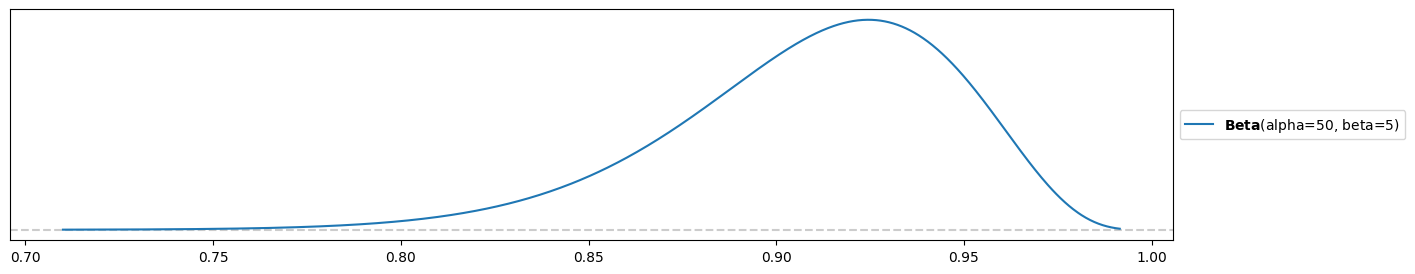

Have reached the desired prior only approximately using the beta distribution! It could allow for a bit more room towards 100%.

e) Sal (who is a touch hyperbolic) just interviewed for a job, and doesn’t know how to describe their chances of getting an offer. They say: “I couldn’t read my interviewer’s expression! I either really impressed them and they are absolutely going to hire me, or I made a terrible impression and they are burning my resumé as we speak.”

This calls for a beta distribution with $\alpha, \beta < 1$ !

pz.Beta( alpha=0.8, beta=0.8 ).plot_pdf()
plt.yticks(np.arange(0,7,1));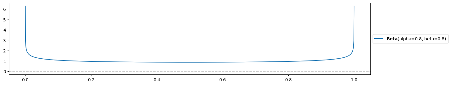

Exercise 2: Älplermagronen¶

Heidi and Peter both like Älplermagronen very much (Swiss dish with maccheroni, potatos, onions, cream, a lot of cheese and apple puré). However, they strongly disagree and often argue about one critical point: whether the apple puré should be mixed with the rest or be served separately.

Heidi who does not like mixing says: “I’m very sure that almost nobody mixes the apple puré with the rest! I would say that around 5% of the population are doing it, maybe up to 10%, but certainly not 20%!”
Peter who likes it very much argues: “I do not believe this! I would guess that the ratio is about fifty-fifty!” (he seems however less sure in his statement than Heidi).

Soonafter, Peter participates in a dinner, where he is the only one out of 6 people who mixes their apple puré with the rest.

a) What conjugate family do you choose to model the proportion $q$ of the Swiss population that mixes their apple puré with the rest? Elicit priors that reflect the opinions of Heidi and Peter well and visualize them (e.g. with Preliz).

Use beta-binomial family!

Prior for Heidi by iteratively trying a few values for $\alpha$ and $\beta$ (might be slightly different from yours):

alpha_heidi = 3
beta_heidi = 35
pz.Beta(alpha=alpha_heidi, beta=beta_heidi).plot_pdf()

<Axes: >

Prior for Peter (again, you might differ):

alpha_peter = 20
beta_peter = 20
pz.Beta(alpha=alpha_peter, beta=beta_peter).plot_pdf()

<Axes: >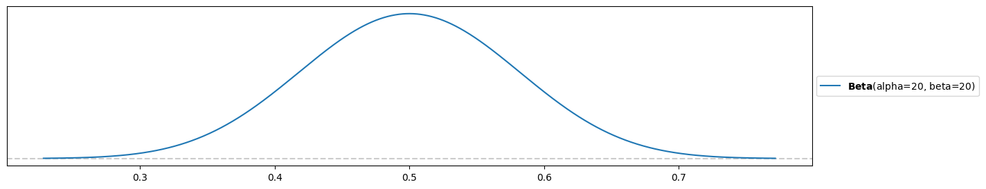

b) Compute the parameters of Heidi and Peter’s posterior distributions. How do their opinions change in the light of data? Compare to their prior distributions.

Experiment (dinner):

n = 6
k = 1

Heidi’s posterior

pz.Beta(alpha=alpha_heidi, beta=beta_heidi).plot_pdf()
pz.Beta(alpha=alpha_heidi+k, beta=beta_heidi+n-k).plot_pdf()
plt.title("Evolution of Heidi's opinion (blue: prior, orange: posterior)")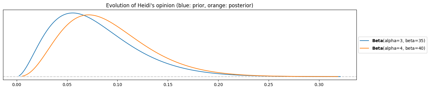

The change is almost not visible! Compare prior and posterior means:

pz.Beta(alpha=alpha_heidi, beta=beta_heidi).mean(), pz.Beta(alpha=alpha_heidi+k, beta=beta_heidi+n-k).mean()

(0.07894736842105263, 0.09090909090909091)

A marginal move towards higher percentages from 8% to 9%.

Peter’s posterior

pz.Beta(alpha=alpha_peter, beta=beta_peter).plot_pdf()
pz.Beta(alpha=alpha_peter+k, beta=beta_peter+n-k).plot_pdf()
plt.title("Evolution of Peter's opinion (blue: prior, orange: posterior)")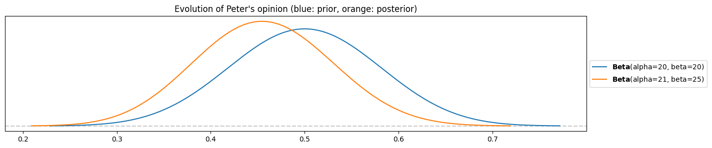

The move is a bit stronger towards lower ratios. Means:

pz.Beta(alpha=alpha_peter, beta=beta_peter).mean(), pz.Beta(alpha=alpha_peter+k, beta=beta_peter+n-k).mean()

(0.5, 0.45652173913043476)

His mean belief went from 50% to 46%.

c) How much would it change for Heidi’s posterior opinion if instead of just Peter all of the 6 participants would have mixed? Could Peter convince her with this data? If no, how many people would they have needed to be (all mixing) to increase the expectation of Heidi’s opinion to at least 50%?

k = 6
pz.Beta(alpha=alpha_heidi, beta=beta_heidi).plot_pdf()
pz.Beta(alpha=alpha_heidi+k, beta=beta_heidi+n-k).plot_pdf()
plt.title("Evolution of Heidi's opinion if all 6 people would have mixed (blue: prior, orange: posterior)")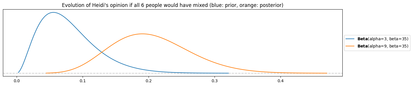

Heidi would move to a mode/average of almost 20%! This is a big change for her, however she is still far away from being convinced by Peter.

What number of people who all mix their apple puré would be necessary to put her posterior mean up to 50%?

With preliz:

n_range = np.arange(6, 40)
posterior_means = np.array( [pz.Beta(alpha=alpha_heidi+n, beta=beta_heidi+n-n).mean() for n in n_range] ) # n=k
plt.plot( n_range, posterior_means )
plt.axhline( 0.5, c="black", ls="--" )
plt.title("$E[\pi] > 0.5$ for $n > {}$".format(6+np.argmax(posterior_means > 0.5)));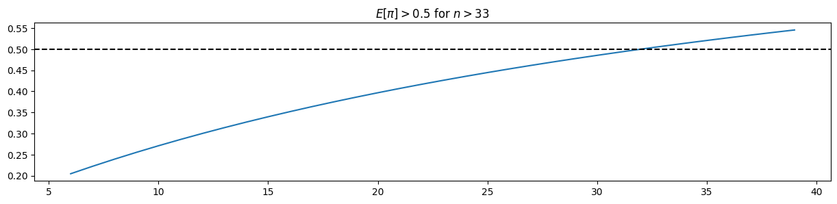

with pandas:

df = pd.DataFrame({'n': n_range, 'posterior_mean': posterior_means})
df[df.posterior_mean > 0.5]

Loading...

To convince Heidi, 33 people would have needed to attend the dinner and mix their apple puré with the rest!

Exercise 3: Maths of the beta-binomial family¶

In this exercise, you are going to explore some of the maths of the beta-binomial family, just to get to know its inner workings a bit better.

a) The beta-family of distributions parameterized by $\alpha$ and $\beta$ is given by:

p(\pi;\alpha,\beta)=\frac{\Gamma(\alpha+\beta)}{\Gamma(\alpha)\Gamma(\beta)}\pi^{\alpha-1}(1-\pi)^{\beta-1}

(4)

Compute its mean $E[\pi]=\int_{0}^{1}\pi~p(\pi;\alpha,\beta)d\pi.$ Hints: Use that $\int_{0}^{1}p(\pi;\alpha,\beta)d\pi=\frac{\Gamma(\alpha)\Gamma(\beta)}{\Gamma(\alpha+\beta)}$ and that $\Gamma(z+1)=z~\Gamma(z)$ .

\begin{align*} E[\pi] &= \int_0^1 \pi \; p(\pi; \alpha, \beta) \; \text{d}\pi = \int_0^1 \pi \; \frac{\Gamma(\alpha+\beta)}{\Gamma(\alpha)\; \Gamma(\beta)} \; \pi^{\alpha-1} \; (1-\pi)^{\beta-1} \; \text{d}\pi\\ &= \frac{\Gamma(\alpha+\beta)}{\Gamma(\alpha)\; \Gamma(\beta)} \; \int_0^1 \pi^{\alpha} \; (1-\pi)^{\beta-1} \; \text{d}\pi\\ &= \frac{\Gamma(\alpha+\beta)}{\Gamma(\alpha)\; \Gamma(\beta)} \; \frac{\Gamma(\alpha+1) \; \Gamma(\beta)}{\Gamma(\alpha+\beta+1)} = \frac{\Gamma(\alpha+\beta)}{\Gamma(\alpha)} \; \frac{\Gamma(\alpha+1)}{\Gamma(\alpha+\beta+1)}\\ &= \frac{\Gamma(\alpha+\beta)}{\Gamma(\alpha)} \; \frac{\alpha \; \Gamma(\alpha)}{(\alpha+\beta) \; \Gamma(\alpha+\beta)}\\ &= \frac{\alpha}{\alpha+\beta} \end{align*}

(5)

b) If a $Beta(\alpha, \beta)$ prior is used and $n$ experiments are run, resulting in $k$ positive outcomes, then we update our belief to a $Beta(\alpha+k,\beta+n-k)$ posterior.

Show that the posterior mean $E[\pi|Y=k]$ can be decomposed into a weighted sum of the prior mean $E[\pi]$ and the empirical mean $\overline{y}=\frac{k}{n}$ :

E[\pi|Y=k]=\frac{\alpha+\beta}{\alpha+\beta+n}E[\pi]+\frac{n}{\alpha+\beta+n}\overline{y}.

(6)

Hint: Make the ansatz

\underbrace{\frac{\alpha+k}{\alpha+\beta+n}}_{E[\pi|Y=k]} = w \underbrace{\frac{\alpha}{\alpha+\beta}}_{E[\pi]} + (1-w)\frac{k}{n},

(7)

solve for $w$ and compute $1-w$ .

\frac{\alpha+k}{\alpha+\beta+n} = w \; \frac{\alpha}{\alpha+\beta} + (1-w) \; \frac{k}{n}

(8)

\Rightarrow \frac{\alpha+k}{\alpha+\beta+n} = w \; \left( \frac{\alpha}{\alpha+\beta} - \frac{k}{n} \right) + \frac{k}{n}

(9)

w = \frac{\frac{\alpha+k}{\alpha+\beta+n} - \frac{k}{n}}{\frac{\alpha}{\alpha+\beta} - \frac{k}{n}} = \frac{\frac{\alpha n + k n - \alpha k - \beta k - nk}{n(\alpha+\beta+n)}}{\frac{\alpha n - k\alpha -k\beta}{(\alpha+\beta) n}} = \frac{\alpha n - \alpha k - \beta k}{\alpha+\beta+n} \; \frac{\alpha+\beta}{\alpha n - \alpha k - \beta k} = \frac{\alpha+\beta}{\alpha+\beta+n}

(10)

1-w = 1 - \frac{\alpha+\beta}{\alpha+\beta+n} = \frac{\alpha+\beta+n}{\alpha+\beta+n} - \frac{\alpha+\beta}{\alpha+\beta+n} = \frac{n}{\alpha+\beta+n}

(11)

c) What are the limits $\lim_{n\rightarrow0}E[\pi|Y=k]$ and $\lim_{n\rightarrow\infty}E[\pi|Y=k]$ ?

Give an interpretation. How do you need to choose $\alpha$ and $\beta$ such that data dominate less for large $n$ ?

$\displaystyle{\lim_{n\to 0}} \; E[\pi|Y=k] = E[\pi]\quad$ (prior dominates the posterior mean)
$\displaystyle{\lim_{n\to \infty}} \; E[\pi|Y=k] = \bar{y}\quad$ (empirical mean dominates the posterior mean)

large $n$ dominate less if $\alpha$ and $\beta$ (and consequently $\alpha+\beta$ are also large. This is equivalent to a strong prior (the larger $\alpha$ and $\beta$ , the smaller the variance). It makes sense that it takes more data to convince a strong prior than it takes to convince a weak prior (with small values for $\alpha$ and $\beta$ ).

Exercise 4: Playing around with your magic coin¶

The posterior is a balance between the prior and the data (through likelihood). In this exercise you will run some simulations to demonstrate this.

You have bought a magic coin with inherent long-run probability for heads $\pi=0.7$ . This is indicated on the wrapping and you got assured by the magic store owner that this value can be trusted (in the long-run of course). You choose to play a bit around with the magic coin to explore the properties of the beta-binomial conjugated family.

a) Create three datasets by running three simulations with $n_{1}=10$ , $n_{2}=100$ and $n_{3}=30$ coin tosses.

Store the values of $k$ (that vary each time you re-run the code). Compute the frequentist estimate $\hat{\pi}_{i}=\frac{k_{i}}{n_{i}}$ for each dataset.

Simulation:

n1 = 10; n2 = 30; n3 = 100
pi_true = 0.7
k1 = np.sum( np.random.choice([0,1], p=[1-pi_true, pi_true], size=n1) )
k2 = np.sum( np.random.choice([0,1], p=[1-pi_true, pi_true], size=n2) )
k3 = np.sum( np.random.choice([0,1], p=[1-pi_true, pi_true], size=n3) )

Frequentist estimate:

k1/n1, k2/n2, k3/n3

(0.8, 0.7, 0.68)

b) You want to try four different priors - Visualize the following four priors using e.g. Preliz!

Uniform, uninformed prior: $Beta(1,1)$

alpha1 = beta1 = 1
pz.Beta(alpha1, beta1).plot_pdf()

<Axes: >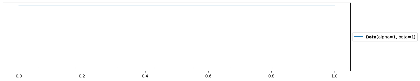

Weakly-informed prior: $Beta(10,4.5)$

alpha2 = 10
beta2 = 4.5
pz.Beta(alpha2, beta2).plot_pdf( support="full" )

<Axes: >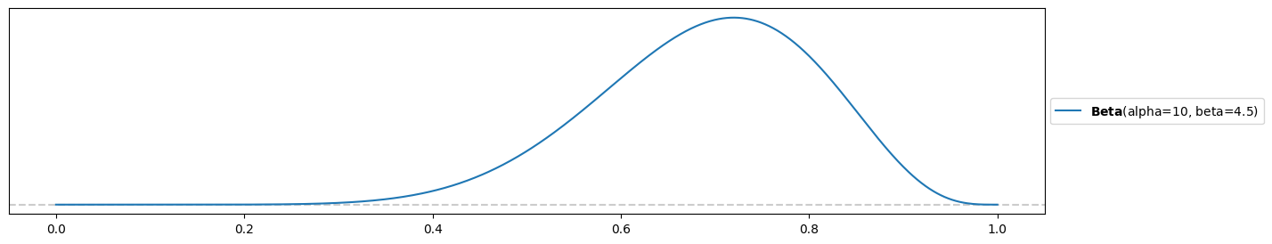

Strongly-informed prior: $Beta(184, 80)$

alpha3 = 184
beta3 = 80
pz.Beta(alpha3, beta3).plot_pdf( support="full" )

<Axes: >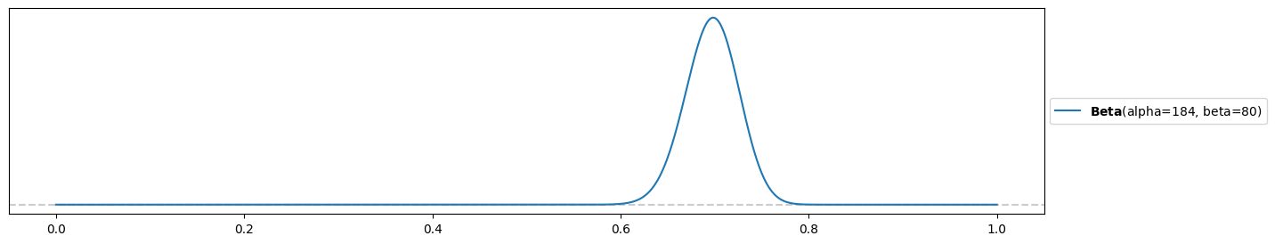

Strongly-informed, wrong prior: $Beta(80, 184)$

alpha4 = 80
beta4 = 184
pz.Beta(alpha4, beta4).plot_pdf( support="full" )

<Axes: >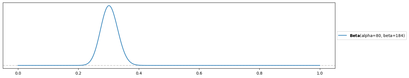

c) Copy the function plot_beta_binomial() from week2_tongue_rolling.ipynb (week 2 materials) to your notebook and run the definition so that you have access to it later.

Now create three plots using plot_beta_binomial() for the three different datasets using the uninformed $Beta(1,1)$ prior. Can you reproduce some conclusions from the lecture? Do the same for the weakly-informed, the strongly-informed and the wrong, strongly-informed prior and provide comments to what you observe.

Since you sampled the coin tosses randomly, you may re-run the cells for this exercise in your notebook—you may be surprised how some results vary by quite a bit!

Use function from tongue rolling notebook:

from scipy import stats

def plot_beta_binomial( alpha, beta, n, k, figsize=(13,3) ):
    # create figure
    plt.figure( figsize=figsize )
    
    # numeric evaluation range for pi
    pi_range = np.linspace(0, 1, 1000)
    
    # prior
    prior = [stats.beta.pdf(pi, a=alpha, b=beta) for pi in pi_range]
    plt.plot( pi_range, prior, alpha=0.5, label="prior", c="orange" )
    plt.fill_between( pi_range, prior, alpha=0.3, color="orange" )

    # scaled likelihood
    likelihood = [stats.binom.pmf(n=n, k=k, p=pi) for pi in pi_range]
    likelihood /= np.sum( likelihood ) * (pi_range[1]-pi_range[0])
    plt.plot( pi_range, likelihood, alpha=0.5, label="(scaled) likelihood", c="blue" )
    plt.fill_between( pi_range, likelihood, alpha=0.3, color="blue" )

    # posterior
    posterior = [stats.beta.pdf(pi, a=alpha+k, b=beta+n-k) for pi in pi_range]
    plt.plot( pi_range, posterior, alpha=0.5, label="posterior", color="darkgreen" )
    plt.fill_between( pi_range, posterior, alpha=0.3, color="darkgreen" )
    
    # enable legend and set descriptive title
    plt.legend( fontsize=14 )
    plt.title( "$\\alpha = {}, \; \\beta={}, \; n={}, \; k={}$".format(alpha, beta, n, k) )

For uniform prior:

for i, (n,k) in enumerate( [(n1,k1),(n2,k2),(n3,k3)] ):
    plot_beta_binomial( alpha1, beta1, n, k )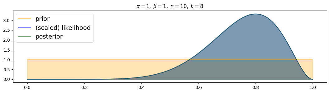

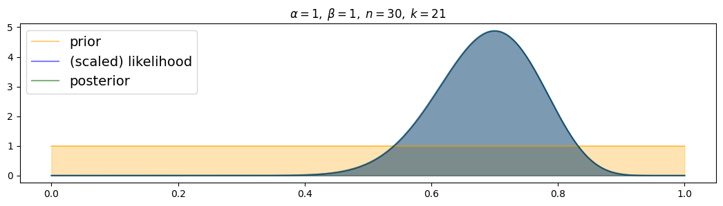
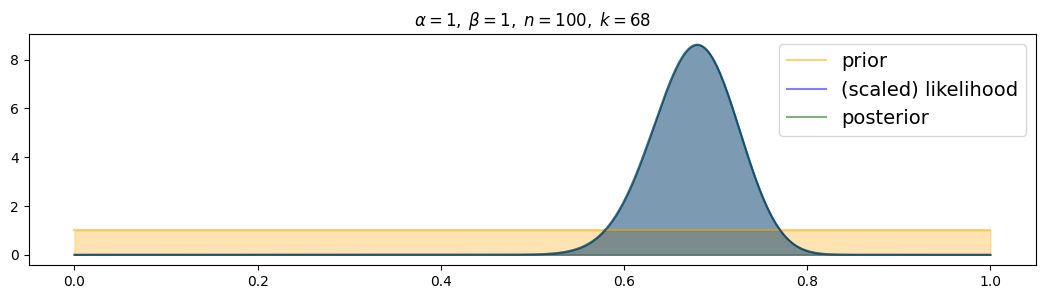
The more data, the more narrow the posterior! (and the closer to the true value)

For weakly-informed prior:

for i, (n,k) in enumerate( [(n1,k1),(n2,k2),(n3,k3)] ):
    plot_beta_binomial( alpha2, beta2, n, k )

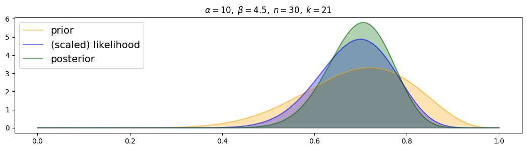
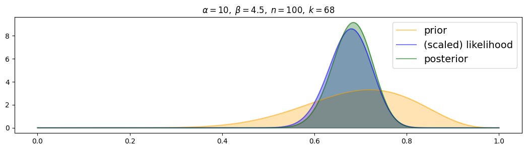
The posterior is always distributed as a compromise between prior and (scaled) likelihood. For more data, the posterior is drawn more to the scaled likelihood and narrower.

For strongly-informed prior:

for i, (n,k) in enumerate( [(n1,k1),(n2,k2),(n3,k3)] ):
    plot_beta_binomial( alpha3, beta3, n, k )

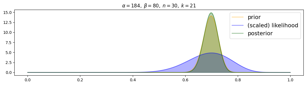
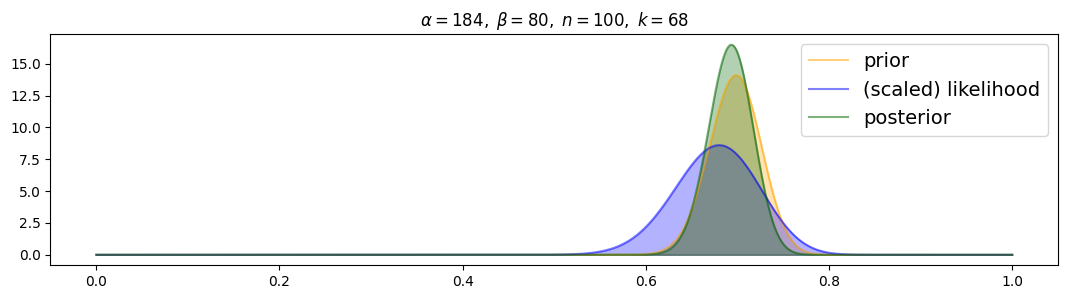
Posterior is drawn to prior from the beginning! Even with 100 samples the prior still dominates the likelihood.

For wrong, strongly-informed prior:

for i, (n,k) in enumerate( [(n1,k1),(n2,k2),(n3,k3)] ):
    plot_beta_binomial( alpha4, beta4, n, k )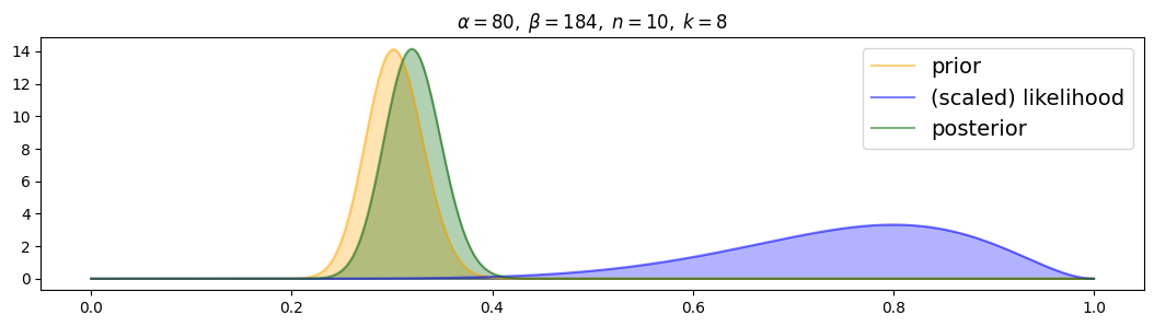

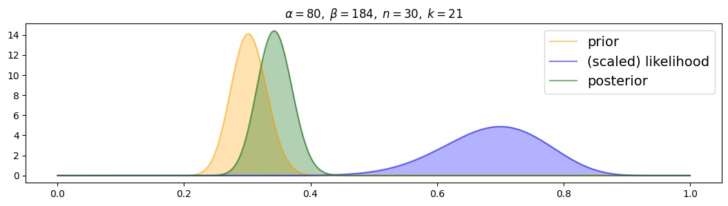
The wrong prior strongly attracts the posterior, with more data it is only slowly attracted towards the likelihood.

Exercise 5: Exam absence¶

A lecturer wants to model the number of absences due to sickness at the final exam of a linear algebra module. He conducted the following measurements so far (HS = Herbstsemester, FS = Frühlingssemester):

Semester	Absences
HS 19	0
FS 20	2
HS 20	NA
FS 21	5
HS 21	2
FS 22	1
HS 22	0
FS 23	1
HS 23	1
FS 24	2

In HS 20, the students were relieved of the exam during the onset of the Covid-19 pandemic.

a) Due to previous experiences (however without recording data), he thinks that typically one absence needs to be expected and that he will probably not reach the maximum of 5 again (during the pandemic). Use a library such as Preliz to devise an appropriate gamma distribution that reflects this prior opinion.

Try out different values using preliz (note that they use $\alpha$ instead of $s$ and $\beta$ instead of $r$ ):

s = 2
r = 1
pz.Gamma(s, r).plot_pdf()
plt.xlim(-0.5,8)

(-0.5, 8.0)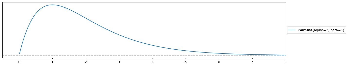

(your prior should look similar but your values for $s$ and $r$ might differ!)

b) What’s the lecturer’s posterior distribution for the number of absences? Use the gamma-Poisson conjugate family and its update rule. Compute also posterior mean, mode and standard deviation as summaries.

y = [0,2,5,2,1,0,1,1,2]

Update rule: $\text{Gamma}(s, r) \to \text{Gamma}(s+\sum_i y_i, r+n)$

Plot prior and posterior:

pz.Gamma(s, r).plot_pdf()
pz.Gamma(s+np.sum(y), r+len(y)).plot_pdf()
plt.xlim(-0.5,8)
plt.title("blue: prior, orange: posterior")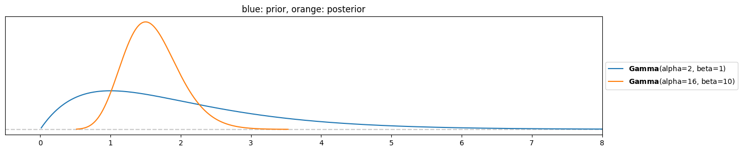

pz.Gamma(s+np.sum(y), r+len(y)).summary()

Gamma(mean=1.6, median=1.57, std=0.4, lower=0.88, upper=2.36)

c) Unlike the lecturer, you do not trust closed-form maths and want to do a simulation to compute posterior mean and standard deviation. You plan to implement it in a similar way as you simulated a beta-binomial posterior in the previous exercise:

Draw $N=10'000$ samples $\lambda_{i}$ from the prior distribution.
Draw 9 samples of absences $k$ for each $\lambda_{i}$ using a Poisson likelihood (same sample number as in provided data).
Filter out only samples that are the same as recorded data (order doesn’t matter, you may use sorting).

Argue that this simulation is very inefficient and might not produce the results you desire, getting even worse if you collect more data. Code is not required, you might nevertheless try it!

Let’s demonstrate this!

Draw samples from prior:

N = 10000
lmbd_vals = pz.Gamma(s, r).rvs(N)
lmbd_vals.shape

(10000,)

Draw 9 Poisson samples for each lambda and sort them, as order does not matter:

samples = [sorted(list(pz.Poisson(mu=lmbd).rvs(9))) for lmbd in lmbd_vals]
samples[:10]

[[1, 2, 2, 2, 3, 3, 5, 6, 6],
 [1, 3, 3, 3, 5, 5, 5, 7, 7],
 [0, 1, 2, 2, 2, 2, 3, 4, 6],
 [0, 0, 0, 1, 1, 1, 1, 2, 3],
 [1, 2, 2, 2, 3, 4, 4, 5, 5],
 [0, 0, 1, 1, 2, 2, 2, 2, 2],
 [0, 1, 2, 2, 2, 3, 3, 3, 3],
 [0, 1, 1, 2, 2, 2, 2, 4, 5],
 [0, 0, 0, 0, 0, 0, 0, 1, 2],
 [0, 0, 0, 1, 1, 1, 1, 2, 3]]

match = [s == sorted(list(y)) for s in samples]
lmbd_vals[match]

array([1.23681577, 1.87586495, 2.01457517, 2.06743204, 1.83493611,
       1.10621502, 1.60273255, 1.07602268, 1.89887354])

This is a very small number of samples to estimate a mean, a standard deviation or even a probability distribution!

np.mean( lmbd_vals[match] ), np.std( lmbd_vals[match] )

(1.6348297588666443, 0.3727309421232923)

Interestingly the values are nontheless not too far away. Nevertheless, this probably gets much worse if we collect more data..

Conclusion: Need a much more effective sampler! (MCMC - next week)

Exercise 6: Empirical Bayes¶

For ‘original’ Bayesians the case is clear: the prior comes before any data and it is not allowed to leak any information from the data into the prior! (you could compare this with leaking test data into a training set in machine learning).

However, there is not just one faction of Bayesians. Empirical Bayesians (calling their approach empirical Bayes) argue that it does not matter so much if enough data are provided and only summaries of the data are used as input to the prior. In this exercise you will use such an ansatz to solve the previous exercise without the need to ‘painfully’ elicit a prior before (it will get worse, you just had to do it for one parameter—what about a regression model with 40 parameters?).

a) Expectation and variance of the gamma distribution are given as

\mu=E[\lambda]=\frac{s}{r} \quad \sigma^{2}=Var[\lambda]=\frac{s}{r^{2}}

(12)

Compute $s$ and $r$ as a function of $\mu$ and $\sigma$ .

Compute formulas for $s$ and $r$ given $\mu$ and $\sigma^2$ :

$\mu = \frac{s}{r} \quad \Rightarrow s = r \; \mu$

$\sigma^2 = \frac{s}{r^2} = \frac{\mu}{r} \quad \Rightarrow r = \frac{\mu}{\sigma^2}$

b) Compute $\mu$ and $\sigma$ from the data (see previous exercise) and create and visualize the resulting empirical prior and compare it to your prior distribution elicited in the previous exercise.

Compute $\mu$ and $\sigma^2$ from data:

mu = np.mean( y )
var = np.var( y )

r_emp = mu/var
s_emp = r_emp * mu
r_emp, s_emp

(0.7682926829268291, 1.195121951219512)

Compare priors:

pz.Gamma( s, r ).plot_pdf()
pz.Gamma( s_emp, r_emp ).plot_pdf()

<Axes: >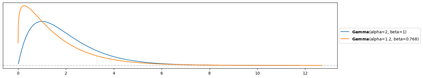

The empirical prior is a bit more right-skewed and concentrated on lower numbers of absences.

c) Use the data to update your prior and visualize the resulting posterior. Compare it to the posterior you got in the previous exercise. How big is the difference? Should you curse empirical Bayesians or do they maybe have a point to make a Bayesian analysis a bit less rigoros but more simple?

Compare posteriors:

pz.Gamma( s+np.sum(y), r+len(y) ).plot_pdf()
pz.Gamma( s_emp+np.sum(y), r_emp+len(y) ).plot_pdf()

<Axes: >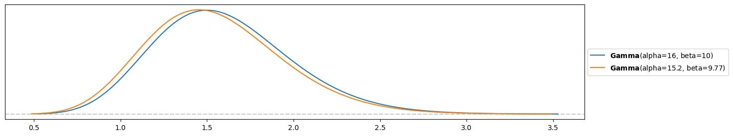

The posteriors are however very similar, maybe empirical Bayes has a point.. Given enough data points (10 in this case), the posterior is already quite robust against small changes in the prior. This would of course be different, if the elicited prior from the previous exercise and the empirical Bayes prior from this exercise would differ significantly!