Gaussian Processes
Definition
Weight-Space View vs. Function-Space View
Source
import gaussian_linear_regression as glr

# =====================================================
# Gaussian Process with linear kernel
# =====================================================

def linear_kernel(Xp, S):
    return Xp @ S @ Xp.T

def generate_gp_samples(mean, K, M):
    N = len(mean)
    L = np.linalg.cholesky(K + 1e-8*np.eye(N))
    Z = np.random.randn(N, M)
    return mean[:,None] + L @ Z   # -> (N,M)


# =====================================================
# COMBINED 3-PANEL PLOT
# =====================================================

def plot_wv_fv(M):

  # =====================================================
  # PRIOR SETTINGS
  # =====================================================

  m = np.zeros((2,1))
  S = np.eye(2)*[0.00001,0.1]

  b_array = np.linspace(-1,1,200)
  a_array = np.linspace(-0.03,0.03,200)
  A, B = np.meshgrid(a_array, b_array)

  Z = np.array([glr.log_prior(ai, bi, m, S) for (ai,bi) in zip(A.ravel(), B.ravel())])
  Z = Z.reshape(len(a_array), len(b_array))

  # Sample weights from prior

  samples = glr.generate_mvn_samples(m, S, M)
  ahat = samples[0,:]
  bhat = samples[1,:]

  # =====================================================
  # GP FUNCTION SPACED SAMPLES WITH LINEAR KERNEL
  # =====================================================

  xp = np.linspace(40, 160, 200)[:,None]
  Xp = np.column_stack([xp[:,0], np.ones(len(xp))])  # (N×2)

  Kpp = linear_kernel(Xp, S)
  gp_samples = generate_gp_samples(np.zeros(len(Xp)), Kpp, M)

  plt.figure(figsize=(18,6))

  # -----------------------
  # LEFT: prior over (a,b)
  # -----------------------
  plt.subplot(1,3,1)
  plt.contour(a_array, b_array, glr.log_to_density(Z), cmap='plasma')
  plt.plot(ahat, bhat, 'bo', ms=6)
  plt.xlabel("slope a")
  plt.ylabel("intercept b")
  plt.title(r"$w \sim \mathcal{N}(0, \Sigma_p)$")
  plt.grid(True)

  # -----------------------
  # MIDDLE: straight lines from prior samples
  # -----------------------
  plt.subplot(1,3,2)
  xp = np.linspace(40, 160, 200)[:,None]
  for a,b in zip(ahat, bhat):
      plt.plot(xp, glr.predict(xp, a, b), color='blue', alpha=0.7)
  plt.title(r"$f=Xw$")
  plt.xlabel("Area")
  plt.ylabel("Price")
  plt.ylim(-1,1)
  plt.grid(True)

  # -----------------------
  # RIGHT: GP samples with linear kernel
  # -----------------------
  plt.subplot(1,3,3)
  plt.plot(xp, gp_samples, color='red', alpha=0.7)
  plt.title(r"$f\sim \mathcal{N}(0, X\Sigma_p X^T)$")
  plt.xlabel("Area")
  plt.ylabel("Price")
  plt.ylim(-1,1)
  plt.grid(True)

  plt.tight_layout()
  plt.show()
  print("Weight samples shape:", samples.shape)
  print("GP samples shape:", gp_samples.shape)

plot_wv_fv(M=4)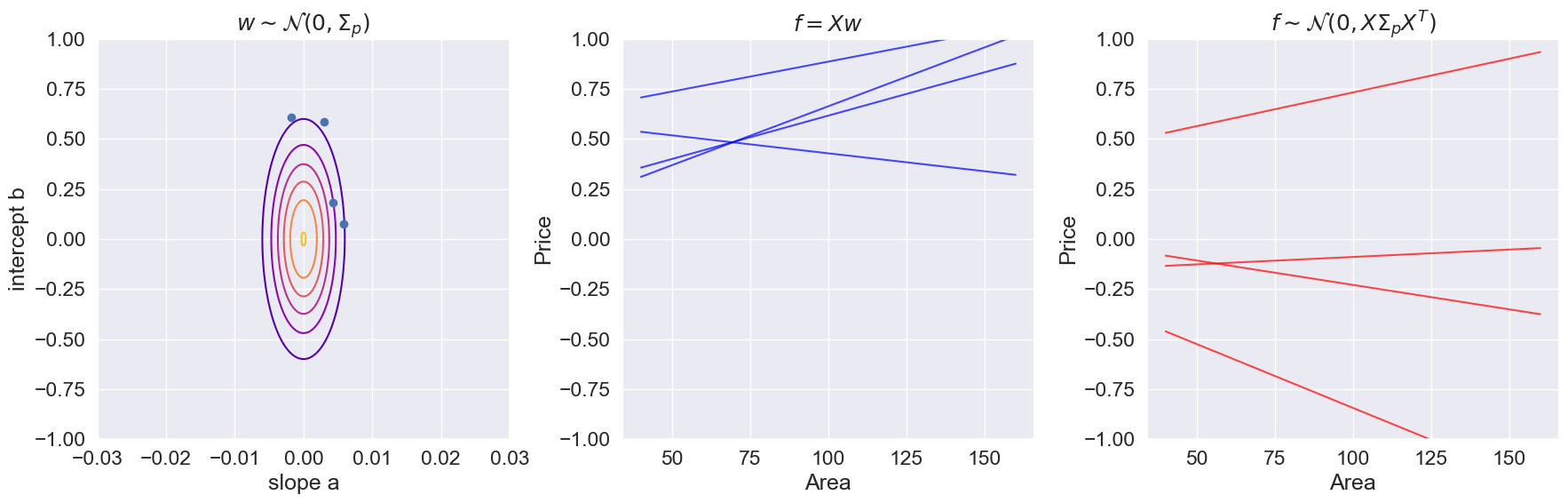
Weight samples shape: (2, 4)
GP samples shape: (200, 4)
Squared exponential kernel (RBF)
The squared exponential covariance function is given by
where and are hyperparameters of the kernel. This specific covariance function is perhaps the most common covariance function used in statistics and machine learning. It is also known as the radial basis function (RBF) kernel, the gaussian kernel, or the exponentiated quadratic kernel.
Below you are given a vector of points on the real line. The points are sorted and equidistantly distributed in the interval .
Notebook Cell
# create an Nx1 vector of equidistant points in [-3, 3]
N = 50
Xp = np.linspace(-3, 9, N)[:, None]
Implement the Kernel
Complete the implementation of the squared exponential kernel function below. (Hint: the code only needs to work with ).
def create_se_kernel(X1, X2, alpha=1, scale=1):
    """ returns the NxM kernel matrix between the two sets of input X1 and X2

    arguments:
    X1    -- NxD matrix
    X2    -- MxD matrix
    alpha -- scalar
    scale -- scalar

    returns NxM matrix
    """
    dist_sq = np.sum((X1[:,None] - X2) **2, axis=2)

    kernel_matrix = alpha * np.exp(-dist_sq / (2 * (scale**2)))
    return kernel_matrix
Compute the Kernel Matrix
Use the kernel function to compute the kernel matrix for the points with and . These points will be used for predictions later and hence, the superscript ‘p’. Visualize the kernel function as an image and give an interpretation of the structure of the kernel. (imshow function)
Kpp = create_se_kernel(Xp, Xp, alpha=1, scale=1)
plt.imshow(Kpp, interpolation='None')
plt.grid(False)
print(f"\nThe RBF matrix shape is {Kpp.shape}")
The RBF matrix shape is (50, 50)
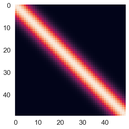
Interpretation of the Kernel Matrix
Try few other parameter values and explain how they affect the structure of the kernel:
Source
fig,ax=plt.subplots(nrows=3, ncols=3, figsize=(20, 20))
alphas = [1, 2, 4]
scales = [1, 2, 4]

X1, X2 = np.meshgrid(Xp, Xp)

for indexAlpha, alpha in enumerate(alphas):
    for indexScale, scale in enumerate(scales):
        K = create_se_kernel(Xp, Xp, alpha, scale)
        cp = ax[indexAlpha][indexScale].imshow(K, interpolation='None')
        ax[indexAlpha][indexScale].grid(False)
        ax[indexAlpha][indexScale].set_title(f"alpha = {alpha}, scale = {scale}")
        #fig.colorbar(cp) # Add a colorbar to a plot
Basically, the RBF kernel tries to measure the similarity between two vectors (Xp and Xp). From the above figure, we can see that the main diagonal has high RBF values, and the value gradually decreases as it moves further away from the diagonal. The distribution of the RBF is a bell-shape (like normal distribution) with the center defined at the point where two elements from the two vectors are exactly equal. The brightest region in the heatmap is called the Region Of Similarity.
How the hyperparameters affect the RBF kernel:
The alpha parameter controls the scaling of the kernel function. A larger value of alpha results in a larger scaling factor, which in turn leads to larger kernel values for all pairs of input vectors. This means that increasing alpha will increase the overall similarity between input vectors, leading to a broader and more diffuse region of similarity. Conversely, decreasing alpha will result in a narrower and more concentrated region of similarity.
The scale parameter controls the width of the Region of Similarity. The larger the scale, the wider this region becomes and vice versa. When the scale is larger, the kernel function will decrease more slowly with distance, resulting in a wider region of similarity. Conversely, a smaller value of ell means that the kernel function will decrease more quickly with distance, resulting in a narrower region of similarity.
Sampling from a Gaussian process
We will consider a zero-mean Gaussian process prior for functions of the form using the squared exponential kernel from the previous section. That is,
Let be the value of the function evaluated at a point .
Furthermore, let be the vector of function values for each of the points of from the previous section.
The Gaussian process prior for becomes
where is the kernel matrix you generated previously.
Implement Sampling
Implement the sampling function.
def generate_samples(mean, K, M):
""" returns M samples from a zero-mean Gaussian process with kernel matrix K
arguments:
K -- NxN kernel matrix
M -- number of samples (scalar)
returns NxM matrix
"""
jitter = 1e-8
L = np.linalg.cholesky(K + jitter * np.identity(len(K)))
zs = np.random.normal(0, 1, size=(len(K), M))
fs = mean + np.dot(L, zs)
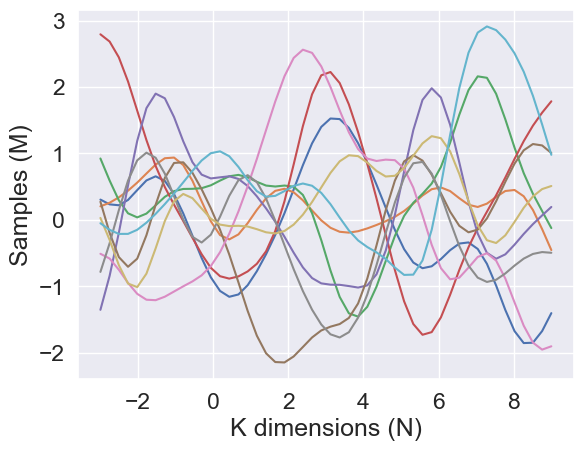
return fsUse Sampling
Generate samples using the new function and plot them.
Source
# Task 3b

# Number of samples
M = 10
# The mean vector
mean = np.zeros(M)

Kpp = create_se_kernel(Xp, Xp, alpha=1, scale=1)
samples = generate_samples(mean, Kpp, M)

print("The sample shape is")
print(samples.shape)

plt.plot(Xp, samples)

# Plotting the samples
plt.ylabel('Samples (M)')
plt.xlabel('K dimensions (N)')
# Show the plot
plt.show()
The sample shape is
(50, 10)
Interpret the Parameters
Change the parameters and explain how they affect the generated samples.
Source
fig,ax=plt.subplots(nrows=3, ncols=3, figsize=(22, 22))
alphas = [0.25, 1, 4]
scales = [0.25, 1, 4]
M_test = 50
mean = np.zeros(M_test)

for indexAlpha, alpha in enumerate(alphas):
    for indexScale, scale in enumerate(scales):
        K = create_se_kernel(Xp, Xp, alphas[indexAlpha], scales[indexScale])
        samples = generate_samples(mean, K, M_test)
        ax[indexAlpha][indexScale].plot(Xp, samples)
        ax[indexAlpha][indexScale].set_title(f"alpha = {alpha}, scale = {scale}")
        ax[indexAlpha][indexScale].set_ylabel('Samples (M)')
        ax[indexAlpha][indexScale].set_xlabel('K dimensions (N)')
        ax[indexAlpha][indexScale].set_ylim((-8, 8))
        #fig.colorbar(cp) # Add a colorbar to a plot
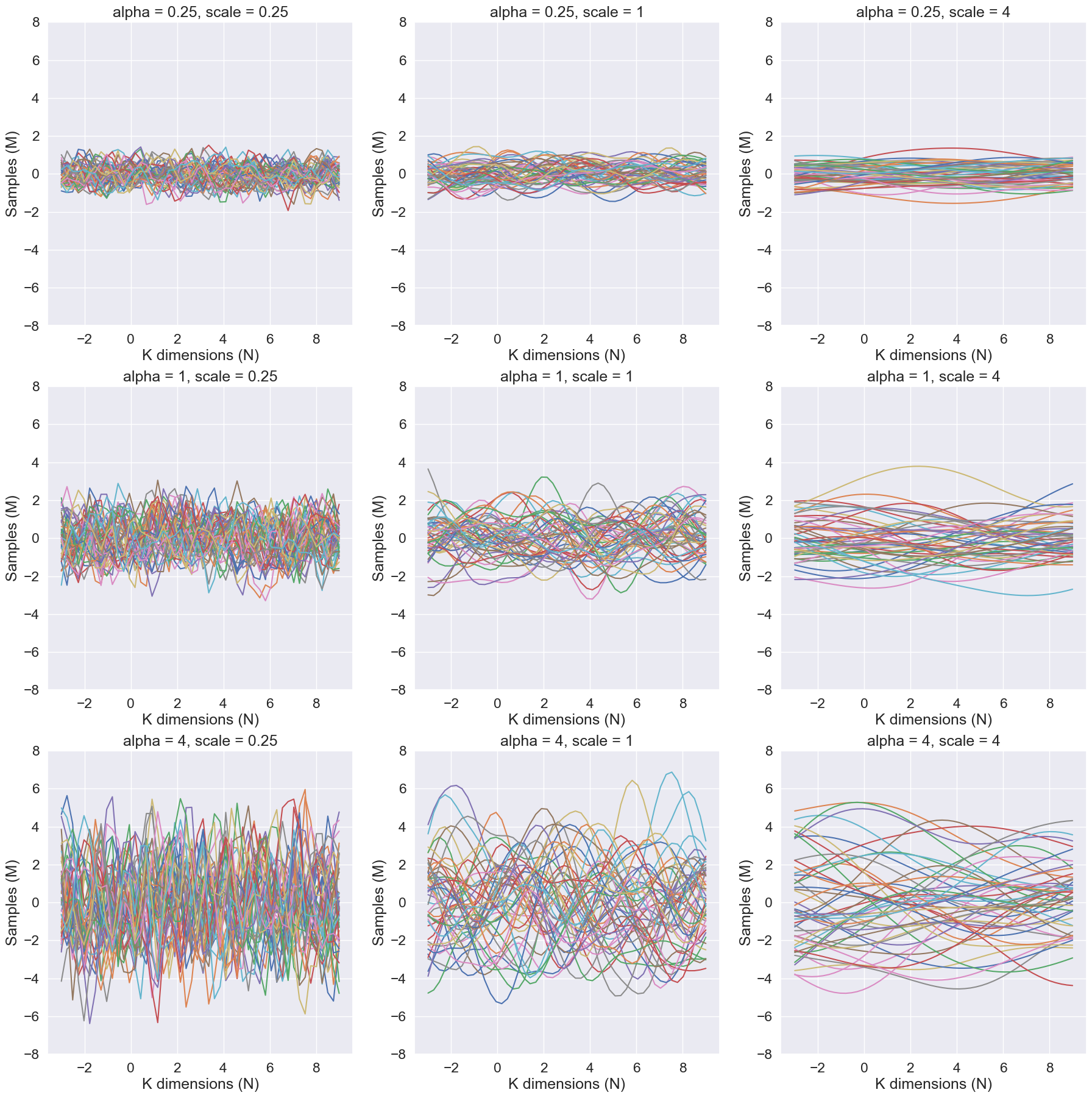
Given a mean of 0 and a covariance matrix defined by the RBF kernel, the hyperparameters alpha and scale affect the distribution of the multivariate samples as follows:
The alpha parameter scales the magnitude of the RBF kernel. A higher value of alpha will result in a covariance matrix with higher variances and stronger correlations between the dimensions. This means that the samples will be more spread out and have a higher correlation between dimensions. This can be seen that as the alpha parameter increases, the samples become similar in pattern along the samples axis
The scale parameter controls the smoothness of the samples. A higher value of scale will result in a covariance matrix with smoother and more gradual changes in the correlation between dimensions. This means that the samples will be less likely to have sudden changes in value between dimensions. This can be seen that as the scale parameter increases, the samples become smoother along the K dimensions axis
The analytical posterior distribution
The goal of this task is complete the implementation of the function below for computing the analytical posterior distribution for a Gaussian process model with Gaussian likelihood, respectively, using the squared exponential kernel.
The joint model for the training data is as follows:
Below you are given a simple toy data set for as visualized below
Source
# load data
data = np.load('data/gaussian-processes.npz')
N = data['N']
X = data['X']
y = data['y']

plt.plot(X, y, 'k.', markersize=12, label='Training data')
plt.grid(True)
plt.xlim((-4, 4))
plt.ylim((-3, 6))
plt.xlabel('Input $x$')
plt.ylabel('Response $y$')
plt.legend()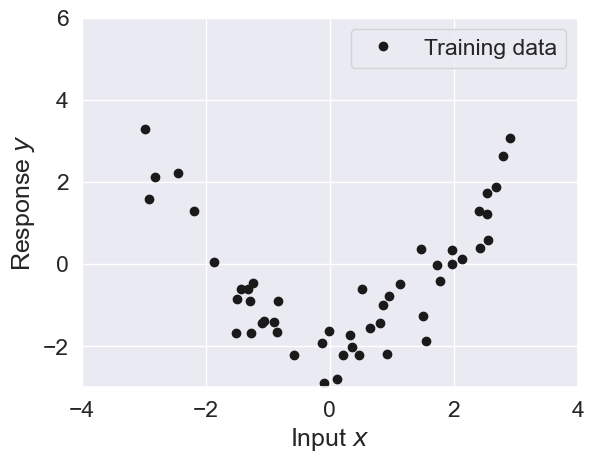
Implement the posterior predictive distribution
Complete the implementation of the function posterior that computes the posterior predictive distribution:
Derivation
The expression above is the posterior predictive distribution of the function given the training data (, ) and the test points :
We assume a latent function with a GP prior:
Using the function we can compute the Kernel matrices for this latent function’s prior:
with – covariances between training points.
with – covariances between test and training points.
with – covariances between test points.
Because we observe noisy instead of , their joint prior is
The the conditional distribution of given is
for:
Implementation
def posterior(Xp, X, y, alpha, scale, sigma2):
    """ returns the posterior distribution of f evaluated at each of the points in Xp conditioned on (X, y)
        using the squared exponential kernel.

    Arguments:
    Xp    -- PxD prediction points
    X     -- NxD input points
    y     -- Nx1 observed values
    alpha -- hyperparameter
    scale -- hyperparameter
    sigma2 -- noise variance

    returns Px1 mean vector and PxP covariance matrix
    """

    K_f_f = create_se_kernel(X, X, alpha=alpha, scale=scale)
    K_fstar_f = create_se_kernel(Xp, X, alpha=alpha, scale=scale)
    K_fstar_fstar = create_se_kernel(Xp, Xp, alpha=alpha, scale=scale)

    post_mu = K_fstar_f @ np.linalg.inv(K_f_f + sigma2 * np.eye(X.shape[0])) @ y
    post_cov = K_fstar_fstar - K_fstar_f @ np.linalg.inv(K_f_f + sigma2 * np.eye(X.shape[0])) @ K_fstar_f.T
    return post_mu, post_cov
Compute the prior & posterior
Compute the prior & posterior of with , , and
sigma2 = 0.5
alpha = 1
scale = 1
Xp = np.linspace(-3, 9, N)[:, None]
print(f"P = {Xp.shape[0]}")
print(f"D = {Xp.shape[1]}")
print(f"N = {X.shape[0]}")

# prior mean and covariance
mu_prior, Sigma_prior = posterior(Xp, np.zeros((0,1)), np.zeros((0,1)), alpha, scale, sigma2)
print(f"Shape of mu_prior is {mu_prior.shape}")
print(f"Shape of Sigma_prior is {Sigma_prior.shape}")
# posterior mean and covariance
mu_post, Sigma_post = posterior(Xp, X, y, alpha, scale, sigma2)
print(f"Shape of mu_post is {mu_post.shape}")
print(f"Shape of Sigma_post is {Sigma_post.shape}")
P = 50
D = 1
N = 50
Shape of mu_prior is (50, 1)
Shape of Sigma_prior is (50, 50)
Shape of mu_post is (50, 1)
Shape of Sigma_post is (50, 50)
Validate Implementation
If the functions above have been implemented correctly, then the following two plots below will show the training data superimposed with prior and posterior, respectively.
Explain what you see in the two figures.
What is the difference between the prior and the posterior in:
regions close to the data points?
in regions far from the data points?
Source
%matplotlib inline
import numpy as np
import pylab as plt


def plot_with_uncertainty(Xp, X, y, n, alpha, scale, sigma2,
                          color='r', color_samples='b',
                          title="", num_samples=0):

    # recompute prior and posterior every time N (n) changes
    mu_prior, Sigma_prior = posterior(Xp,
                                      np.zeros((0,1)),
                                      np.zeros((0,1)),
                                      alpha, scale, sigma2)

    mu_post, Sigma_post   = posterior(Xp,
                                      X[:n, :],
                                      y[:n, :],
                                      alpha, scale, sigma2)

    # choose which version to plot
    if "Prior" in title:
        mu, Sigma = mu_prior, Sigma_prior
    else:
        mu, Sigma = mu_post, Sigma_post

    mean = mu.ravel()
    std  = np.sqrt(np.diag(Sigma))

    # plot distribution
    plt.title(title)
    plt.plot(Xp, mean, color=color)
    plt.plot(Xp, mean + 2*std, color=color, linestyle='--')
    plt.plot(Xp, mean - 2*std, color=color, linestyle='--')
    plt.fill_between(Xp.ravel(),
                     mean - 2*std,
                     mean + 2*std,
                     color=color, alpha=0.25)

    # draw samples if needed
    if num_samples > 0:
        fs = generate_samples(mu, Sigma, num_samples)
        plt.plot(Xp, fs, color=color_samples, alpha=.25)

def plot_data(n):
    plt.plot(X[:n, :], y[:n, :], 'k.', markersize=15, label='Data')
    plt.xlabel('Input x')
    plt.ylim((-5, 5))
    plt.grid(True)

def plot_GP(n):
    plt.figure(figsize=(20, 6))

    # PRIOR
    plt.subplot(1, 2, 1)
    plot_data(n)
    plot_with_uncertainty(Xp, X, y, n,
                          alpha, scale, sigma2,
                          title='Prior distribution',
                          num_samples=10)
    plt.legend(loc='lower right')

    # POSTERIOR
    plt.subplot(1, 2, 2)
    plot_data(n)
    plot_with_uncertainty(Xp, X, y, n,
                          alpha, scale, sigma2,
                          title='Posterior distribution',
                          num_samples=10)
    plt.legend(loc='lower right')

plot_GP(n = 2)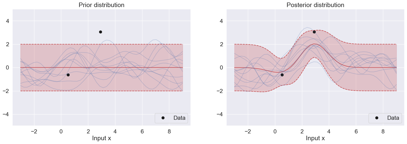
Explain what you see in the two figures
In the first figure, the prior mean is 0, and the prior variance is based on rbf of the testing data. The mean is set at 0 and the confidence level is within the [-2,2] range along the response. This prior is uniformly distributed
In the second figure, the posterior mean follows closely the data pattern from -4 to 4 along the x-input. After that, the posterior starts to resemble the prior again.
What is the difference between the prior and the posterior in
1) regions close to the data points?
The prior is uniform in this region because it does not consider the datapoints.
The posterior takes into account this region and it closely follows the datapoints.
2) in regions far from the data points?
There is no difference between the prior and posterior in regions far from the data points.
Adjust Parameters
Replicate the two figures above for the following three different values of the scale parameter: and for and . Explain the differences between the three sets of plots
Source
def plot_GP(n, scale):
    plt.figure(figsize=(20, 6))

    # PRIOR
    plt.subplot(1, 2, 1)
    plot_data(n)
    plot_with_uncertainty(
        Xp, X, y, n,
        alpha, scale, sigma2,
        title=f'Prior distribution (scale = {scale})',
        num_samples=10
    )
    plt.legend(loc='lower right')

    # POSTERIOR
    plt.subplot(1, 2, 2)
    plot_data(n)
    plot_with_uncertainty(
        Xp, X, y, n,
        alpha, scale, sigma2,
        title=f'Posterior distribution (scale = {scale})',
        num_samples=10
    )
    plt.legend(loc='lower right')

    plt.show()

plot_GP(n = 15, scale = 1)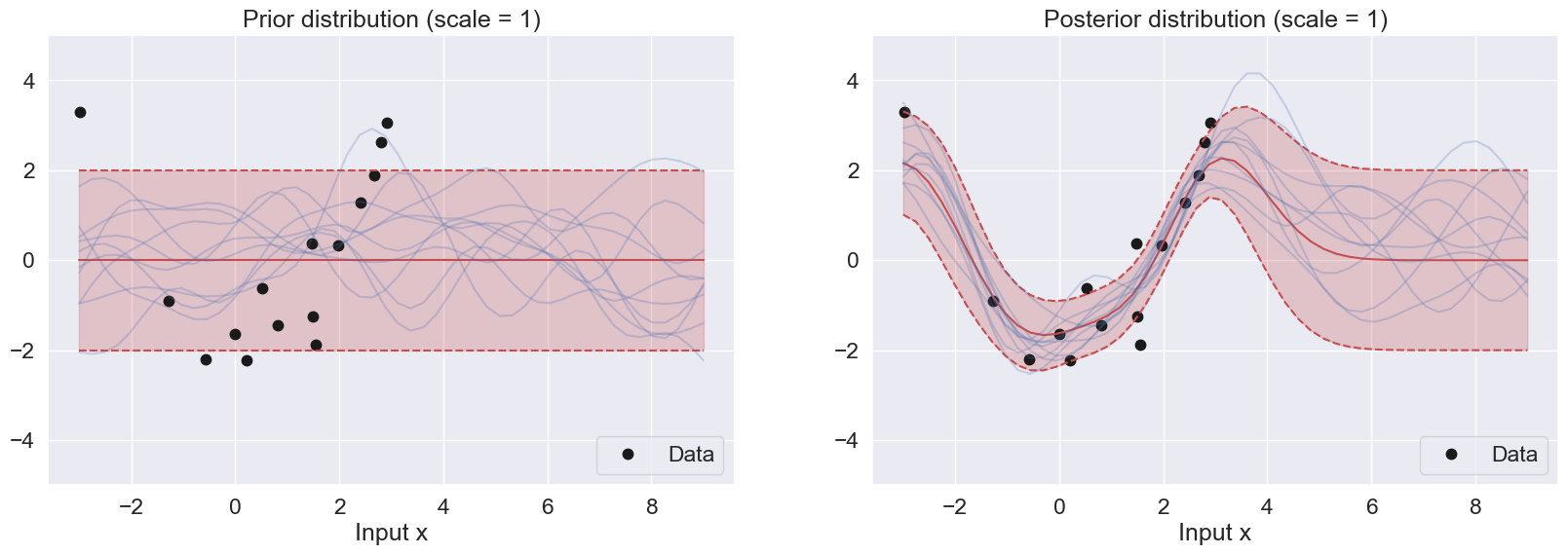
Difference between the figures with different scales:
As described previously, the scale parameter controls the smoothness of the prior samples. As the scale becomes larger, the gradual change between the dimension (Input X) becomes smoother, and as the scale becomes smaller, the samples become highly turbulent. This is observed in the prior distributions above.
For the posterior distributions, a smaller scale leads to a more peaked and narrower posterior distribution, while a larger scale hyperparameter will lead to a flatter distribution. Specifically, if the scale hyperparameter is too small, the GP posterior samples may overfit the training data and have high variance. On the other hand, if the scale hyperparameter is too large, the GP posterior samples may underfit the training data and have high bias
Adjust Sampling
Replicate the two figures above for the following three different values of the alpha parameter: and for and . Explain the differences between the three sets of plots
Source
def plot_GP(n, scale, alpha):
    plt.figure(figsize=(20, 6))

    # PRIOR
    plt.subplot(1, 2, 1)
    plot_data(n)
    plot_with_uncertainty(
        Xp, X, y, n,
        alpha, scale, sigma2,
        title=f"Prior distribution (scale={scale}, alpha={alpha})",
        num_samples=10
    )
    plt.legend(loc='lower right')

    # POSTERIOR
    plt.subplot(1, 2, 2)
    plot_data(n)
    plot_with_uncertainty(
        Xp, X, y, n,
        alpha, scale, sigma2,
        title=f"Posterior distribution (scale={scale}, alpha={alpha})",
        num_samples=10
    )
    plt.legend(loc='lower right')
    plt.show()


plot_GP(n = 50, scale = 1.0, alpha = 0.25)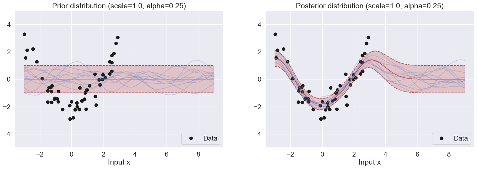
For the prior samples, the alpha parameter controls the magnitude of the samples. When alpha becomes larger, the range of the samples become wider and covers more uncertainty. Smaller alpha results in smaller variance, leading to a narrow range of the samples
For the posterior samples, small alphas try to match the regions with the most concentrated data points while discarding relative outliers. This is because the allowed confidence is small. Larger alphas are able to capture more datapoints because the allowed confidence level is higher.
Marginal Likelihood for Parameter Tuning
The purpose of this task is to study the marginal likelihood and see how it can be useful for model selection. The marginal likelihood for a zero-mean Gaussian process model with Gaussian likelihood is given by
where are the set of hyperparameters, e.g. the alpha and scale parameters for the RBF kernel.
Load Data
First, we will load some validation data that will be useful for evaluating the model.
data = np.load('data/gaussian-processes.npz')Source
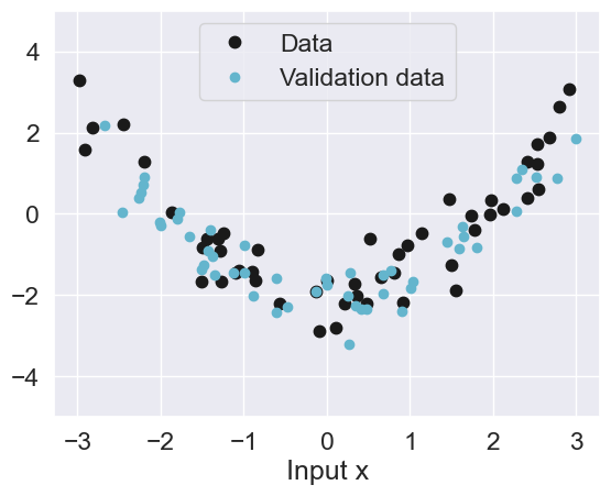
Nval, Xval, yval = data['Nval'], data['Xval'], data['yval']
print(Nval)
plot_data(n=50)
plt.plot(Xval, yval, 'c.', label='Validation data', markersize=12)
plt.legend(loc='upper center');
50
Implement the Posterior Predictive Distribution
Complete the implementation of the function predictive below. The predictive distribution of ‘yp’ combines prediction function posterior (posterior) and the noise variance.
def predictive(Xp, X, y, alpha, scale, sigma2):
    """ returns the predictive distribution of yp
    evaluated at each of the points in Xp conditioned on (X, y)

    Arguments:
    Xp    -- PxD prediction points
    X     -- NxD input points
    y     -- Nx1 observed values
    alpha -- hyperparameter
    scale -- hyperparameter
    sigma2 -- noise variance

    returns Px1 mean vector and PxP covariance matrix
    """


    mu_post, Sigma_post = posterior(Xp, X, y, alpha, scale, sigma2)
    N = len(Xp)
    mu_pred, Sigma_pred = mu_post, Sigma_post + sigma2 * np.eye(N)
    return mu_pred, Sigma_pred
Implement the Mean Log Posterior Predictive Density (MLPPD)
Complete the implementation of the function MLPPD for computing the mean log posterior predictive density given below.
log_pdf = lambda x, m, v: -0.5*(x-m)**2/v -0.5* np.log(2*np.pi*v)

# This function is also known as ELPD (Expected Log Pointwise Predictive Density)
def MLPPD(Xval, yval, mu, Sigma):
    """ returns the mean log posterior predictive density
    for the data points (Xval, yval) wrt. predictive density N(mu, Sigma)

    Arguments:
    Xval      -- PxD input points
    yval      -- Px1 observed values
    mu        -- Px1 mean of predictive distribution
    Sigma     -- PxP covariance of predictive distribution

    Returns
    mlppd     -- (scalar) mean log posterior predictive density

    """

    # Model answer
    var = np.diag(Sigma)
    mlppd = np.mean(log_pdf(yval,mu,var))
    return mlppd
Implement Log Marginal Likelihood
Complete the implementation of the function log_marginal_likelihood given below.
def log_marginal_likelihood(X, y, alpha, scale, sigma2):
""" returns the log marginal likelihood for the data set (X, y) for the hyperparameters alpha, scale, sigma2
The function also returns the components of the log marginal likelihood:
log_ml = const_term + det_term + quad_term
Arguments:
X -- NxD input points
y -- Nx1 observed values
alpha -- alpha parameter
scale -- scale parameter
sigma2 -- noise variance
Returns:
log_ml -- (scalar) log marginal likelihood ( = const + det + quad)
const -- constant part of the log marginal lihood
det -- determinant part of the log marginal lihood
quad -- quadratic part of the log marginal lihood
"""
N = len(X)
K = create_se_kernel(X, X, alpha, scale)
C = K + sigma2 * np.eye(N)
jitter = 1e-8
L = np.linalg.cholesky(C + jitter * np.eye(N))
v = np.linalg.solve(L, y)
const_term = - (N/2) * np.log(2 * np.pi)
det_term = - 0.5 * 2 * np.sum(np.log(np.diag(L)))
quad_term = -(1/2) * np.sum(v ** 2)
log_ml = const_term + det_term + quad_term
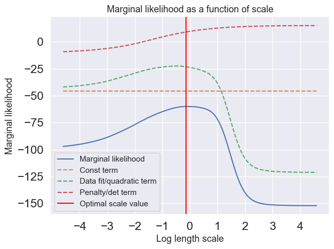
return log_ml, const_term, det_term, quad_termPlot Marginal Likelihood
Compute and plot the marginal likelihood as a function of the scale parameter in the interval using the scales vector (scales) given below. In the same figure, you should also plot the determinant and the quadractic part of the marginal likelihood. Note, that the scale values are distributed equally in log-space. Use and . The scale axis should be logaritmic in the plot. Furthermore, locate the optimal value of the scale and plot the posterior distribution of for the that specific value.
Source
scales = np.logspace(-2, 2, 100)
sigma2=0.5
alpha=1
# Should look like the figure in slide 34
log_ml_list = np.zeros(100)
const_list = np.zeros(100)
det_list = np.zeros(100)
quad_list = np.zeros(100)
for index, scale in enumerate(scales):
log_ml, const_term, det_term, quad_term = log_marginal_likelihood(X, y, alpha, scale, sigma2)
log_ml_list[index] = log_ml
const_list[index] = const_term
det_list[index] = det_term
quad_list[index] = quad_term
log_scales = np.log(scales)
optimal_value_index = np.argmax(log_ml_list)
print(f"The optimal scale value is {scales[optimal_value_index]}")
print(f"Its respective log optimal scale value in the graph is {log_scales[optimal_value_index]}")
plt.figure(figsize=(7, 5))
plt.plot(log_scales, log_ml_list, label="Marginal likelihood")
plt.plot(log_scales, const_list, label="Const term",linestyle="--")
plt.plot(log_scales, quad_list, label="Data fit/quadratic term",linestyle="--")
plt.plot(log_scales, det_list, label="Penalty/det term",linestyle="--")
#plt.xscale('log', base=2)
plt.xticks([-4, -3, -2, -1, 0, 1, 2,3, 4])
plt.title("Marginal likelihood as a function of scale",fontsize=13)
plt.xlabel("Log length scale",fontsize=13)
plt.ylabel("Marginal likelihood",fontsize=13)
plt.axvline(x=log_scales[optimal_value_index], color='red', label="Optimal scale value")
plt.legend(loc=3, fontsize=11)
plt.show()
sigma2=0.5
scale=scales[optimal_value_index]
alpha=1
#mu_prior, Sigma_prior = posterior(Xp, np.zeros((0,1)), np.zeros((0,1)), alpha, scale, sigma2)
#mu_post, Sigma_post = posterior(Xp, X, y, alpha, scale, sigma2)
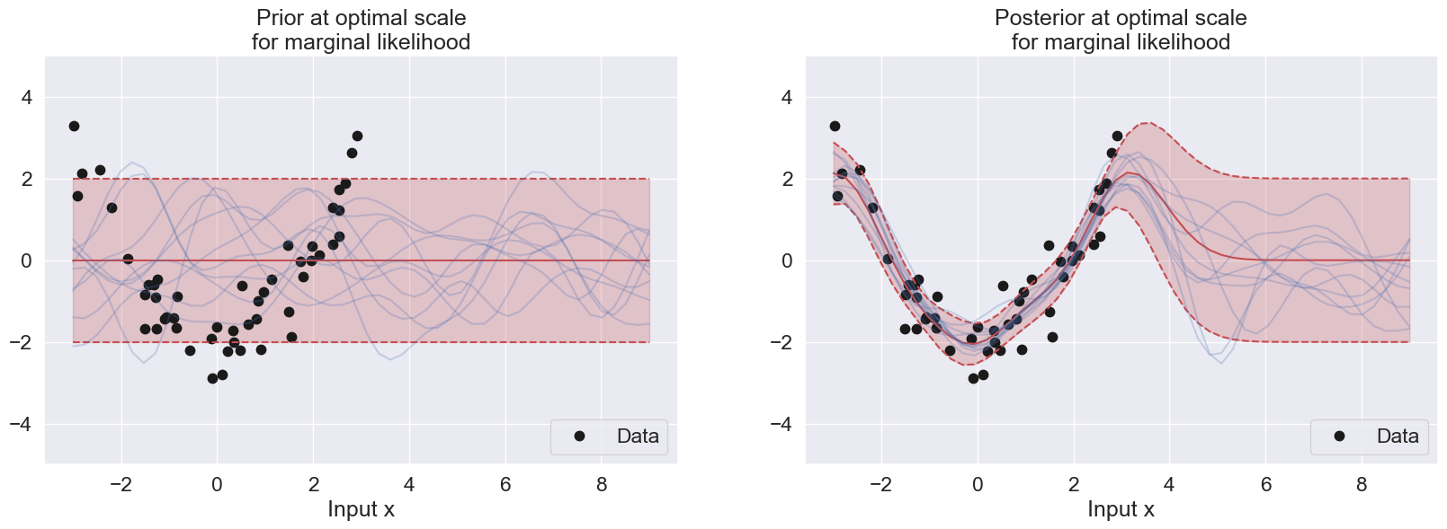
plt.figure(figsize=(20, 13))
plt.subplot(2, 2, 1)
plot_data(50)
plot_with_uncertainty(Xp, X, y, N, alpha, scale, sigma2, title=f'Prior at optimal scale\nfor marginal likelihood', num_samples=10)
plt.legend(loc='lower right')
plt.subplot(2, 2, 2)
plot_data(50)
plot_with_uncertainty(Xp, X, y, N, alpha, scale, sigma2, title=f'Posterior at optimal scale\nfor marginal likelihood', num_samples=10)
plt.legend(loc='lower right')
plt.show()The optimal scale value is 0.8697490026177834
Its respective log optimal scale value in the graph is -0.1395506116966087
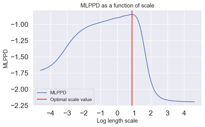
Plot the Mean Log Posterior Predictive Density (MLPPD)
Compute and plot the MLPPD of the validation set as a function of the scale parameter in the interval using the scales vector (scales) given below. Note, the scale values are distributed equally in log-space. Use and . The scale axis should be logaritmic in the plot.
Source
scales = np.logspace(-2, 2, 100)
sigma2=0.5
alpha=1


mlppd_list = np.zeros(100)
for index, scale in enumerate(scales):
    mu_val, Sigma_val = predictive(Xval, X, y, alpha, scale, sigma2)
    mlppd = MLPPD(Xval, yval, mu_val, Sigma_val)
    mlppd_list[index] = mlppd

optimal_value_index = np.argmax(mlppd_list)
print(f"The optimal scale value is {scales[optimal_value_index]}")
print(f"Its respective log optimal scale value in the graph is {log_scales[optimal_value_index]}")

plt.figure(figsize=(7, 4))
plt.plot(log_scales, mlppd_list, label="MLPPD")

#plt.xscale('log', base=2)
plt.xticks([-4, -3, -2, -1, 0, 1, 2,3, 4])
plt.title("MLPPD as a function of scale",fontsize=13)
plt.xlabel("Log length scale",fontsize=13)
plt.ylabel("MLPPD",fontsize=13)
plt.legend(loc=4, fontsize=11)

plt.axvline(x=log_scales[optimal_value_index], color='red', label="Optimal scale value")

plt.legend(loc=3, fontsize=11)
plt.show()


sigma2=0.5
scale=scales[optimal_value_index]
alpha=1

#mu_prior, Sigma_prior = posterior(Xp, np.zeros((0,1)), np.zeros((0,1)), alpha, scale, sigma2)
#mu_post, Sigma_post = posterior(Xp, X, y, alpha, scale, sigma2)

plt.figure(figsize=(20, 13))

plt.subplot(2, 2, 1)
plot_data(N)
plot_with_uncertainty(Xp, X, y, N, alpha, scale, sigma2, title=f'Prior at optimal scale\nfor MLPPD', num_samples=10)
plt.legend(loc='lower right')

plt.subplot(2, 2, 2)
plot_data(N)
plot_with_uncertainty(Xp, X, y, N, alpha, scale, sigma2, title=f'Posterior at optimal scale\nfor MLPPD', num_samples=10)
plt.legend(loc='lower right')

plt.show()
The optimal scale value is 2.4201282647943834
Its respective log optimal scale value in the graph is 0.8838205407451898
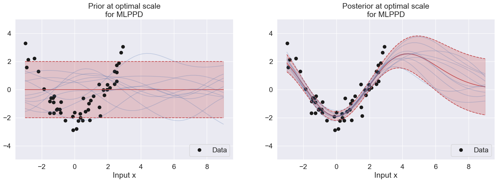
Interpretation of the Plots
The log marginal likelihood and MLPPD can both be used for hyperparameter tuning in Gaussian process regression with an RBF kernel. The difference between them is that the log marginal likelihood is a measure of hyperparameters that maximizes the model fitness on the training data. On the other hand, the MLPPD is a measure of hyperparameters that maximizes the model fitness on new data prediction. As a result, a model with a high log marginal likelihood indicates a good fit to the training data, while a model with a high MLPPD indicates good predictive performance.
In this example, the optimal scale value for MLPPD is much larger than the log marginal likelihood, suggesting that MLPPD prefers larger bias than log marginal likelihood, as MLPPD can be observed to have a smoother transition to static prior region as compared to the log marginal likelihood. This suggests that MLPPD takes into account the future prediction (as its name implies), thus having lower variance than log marginal likelihood (which only aims to fit the training data) and follows the flow of the data pattern.
Exercises
Problem 2.1
Suppose we model the relationship of a real-valued response variable to a single real input, , using a Gaussian process model in which the mean is zero and the covariances of the observed responses are given by:
with the noise-free covariance function defined by:
Suppose we have four training cases, as follows:
| 0.5 | 2.0 |
| 2.8 | 3.3 |
| 1.6 | 3.0 |
| 3.9 | 2.7 |
Recall that the conditional mean of the response in a test case with input , given the responses in the training cases, is
where:
is the vector of observed responses in training cases,
is the vector of responses in test cases,
is the matrix of covariances for the responses in training cases,
is the vector of covariances of the response in the test case with the responses in training cases.
a) Find the predictive mean for the response in a test case in which the input is .
b) Find the predictive mean and variance of the response in a test case in which the input is by means of NumPy.