Bayesian Linear Regression
import pandas as pd
import numpy as np
from scipy import stats
import matplotlib.pyplot as plt
import seaborn as sns
import preliz as pz
import pymc as pm
import arviz as az
import bambi as bmb
plt.rcParams["figure.figsize"] = (8,3)
plt.style.use('ggplot')
np.random.seed(1337) # for consistency
Exercise 1: Modeling Credit Data with Simple Linear Regression
In this exercise, you will perform the basic steps of Bayesian linear regression. To this end, you will work with the credit dataset that you can load with Pandas from credit_data.csv.
credit_data = pd.read_csv("credit_data.csv")
credit_data.head()a)
You would like to predict the balance (current credit card debt in USD) of a person using only the limit set by the bank (in USD) as a predictor. Write down the structure of a linear regression model that achieves this using the mathematical notation from the lecture (priors, likelihood, etc.). Thereby you do not have to specify numeric values for the prior distribution parameters (but you may think about their sizes if you want).
b) Fit a linear regression model with bambi
Fit a linear regression model with bambi, letting it automatically select default priors for you. Extract the model that it created both through backend.model (mathematical notation) and through graph() (graphical model). Does the model align with your own model in a)? If no, what are the differences?
credit_model1 = bmb.Model("Balance ~ Limit", data=credit_data, family="gaussian")
credit_trace1 = credit_model1.fit(draws=2000, tune=2000)credit_model1.backend.modelcredit_model1.graph() # may lead to warnings or errors depending on what versions you use / what packages you have installedBambi uses a half Student’s distribution and I proposed an exponential distribution above. Both only go over positive values and since they are weak there should not be a big difference in the resulting posterior.
c)
Return a summary of the posterior regression coefficient distributions using pm.summary() and plot them visually using pm.plot_posterior() (for both using 95% credible intervals). Write down the mean regression model as a formula. How can the coefficients be interpreted in terms of the effect of the associated predictors on credit card balance?
pm.summary( credit_trace1, hdi_prob=0.95 )pm.plot_posterior( credit_trace1, hdi_prob=0.95 )array([<Axes: title={'center': 'sigma'}>,
<Axes: title={'center': 'Intercept'}>,
<Axes: title={'center': 'Limit'}>], dtype=object)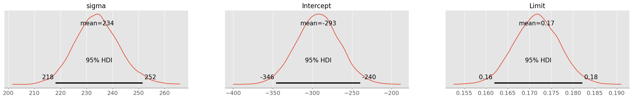
Mean model:
Interpretation: For every USD by that the limit is increased, the customer has 17 cents more debts. However the model does probably not hold for small balances and limits: for a limit of 0, the balance would be -293 USD (intercept). This is probably due to non-linearity.
d)
Create a plot with data and regression line using bmb.interpret.plot_predictions(). Use a 95% HDI for the regression line uncertainty. Using the plot, give an interpretation why the recovered intercept is negative. Also, visually judge aleatoric and epistemic uncertainty.
Hint: Whether bmb.interpret.plot_predictions() plots an HDI of the posterior regression line distribution or of the predictive distribution can be controlled with the pps parameter.
credit_data.plot.scatter( x="Limit", y="Balance" )
bmb.interpret.plot_predictions( credit_model1, credit_trace1, "Limit", prob=0.95, ax=plt.gca() )
(<Figure size 800x300 with 1 Axes>,
array([<Axes: xlabel='Limit', ylabel='Balance'>], dtype=object))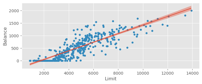
The non-linearity in the beginning is clearly visible, leading to a compensation of the model with a negative intercept.
The epistemic uncertainty is quite small in comparison with the aleatoric certainty (unexplained variance in the data after fitting the model).
e)
How good is your model? Compute the Bayesian predictive versions of RMSE, MAE and score. On this occasion, make sure that you understand the Bayesian interpretation of proposed in the lecture.
credit_model1.predict(credit_trace1, kind="response")
ypred = az.extract( credit_trace1.posterior_predictive ).Balance.values.T
ytrue = credit_data.Balance.values
RMSE:
np.sqrt( np.mean( (ypred - ytrue)**2 ) )np.float64(330.7474098511541)Given the credit card limit, we are able to model the balance by ± 331 USD.
MAE:
np.mean( np.abs( ypred - ytrue ) )np.float64(260.4780826723066)MAE is quite a bit smaller, indicating the presence of points further away from the line than expected.
:
pm.r2_score( ytrue, ypred )r2 0.659406
r2_std 0.018883
dtype: float64The model is doing reasonably well for just one predictor.
f)
You try to predict the balance for a customer with a limit of 3000 USD. Compute the predictive distribution and summarize and visualize it (use a 90% HDI). Does the recovered distribution make sense to you? Give also a summary of its aleatoric and epistemic uncertainty.
Hint: For epistemic and aleatoric uncertainty use predict() on your model and pass your data point to get the predictive distribution conditioned on it. The epistemic uncertainty is the variance of the predicted means and the predictive uncertainty the variance of the predictions for Balance. You may recover the aleatoric uncertainty using .
Compute predictive distribution:
pred = credit_model1.predict( credit_trace1, kind="response", data=pd.DataFrame({'Limit': [3000]}), inplace=False )
pm.summary( pred.posterior_predictive, hdi_prob=0.9 )pm.plot_posterior( pred.posterior_predictive, hdi_prob=0.9 )<Axes: title={'center': 'Balance\n0'}>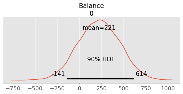
With a probability of 90%, the balance will be between -153 and 618 USD. This is clearly an artefact of a ‘wrong’ likelihood model (normal), since balance (debts) cannot be negative.
var_e = pred.posterior.mu.var().values
var_p = pred.posterior_predictive.Balance.var().values
var_a = var_p - var_e
np.sqrt( var_a ), np.sqrt( var_e ), np.sqrt( var_p )
(np.float64(232.36122763552714),
np.float64(14.903739211518685),
np.float64(232.8387028626775))Ratios:
var_e/var_p, var_a/var_p(np.float64(0.004097133761204795), np.float64(0.9959028662387952))Most of the uncertainty is of aleatoric nature! Collecting more data will not make the model better.
Exercise 2: Alternative Likelihoods
You are a bit frustrated by the negative balances predicted by your model in Exercise 1. You have the brilliant idea to change the likelihood of your model to produce only positive values. Instead of , you choose the likelihood
since the maximum observed balance in your data is 2000.
a)
Since the TruncatedNormal likelihood is not available in Bambi, implement your model in PyMC (slight modification of code used in lecture) and run the posterior simulation.
x = credit_data.Limit
y_obs = credit_data.Balance

with pm.Model() as credit_model2:
    # priors
    beta0 = pm.Normal('beta0', mu=credit_data.Balance.mean(), sigma=10 )
    beta1 = pm.Normal('beta1', mu=0, sigma=10 )
    sigma = pm.Exponential('sigma', lam=1/10 )

    # likelihood
    y = pm.TruncatedNormal('y', mu=beta0+beta1*x, lower=0, upper=2000, sigma=sigma, observed=y_obs )

    # simulate posterior
credit_trace2 = pm.sample( 2000 )b)
Compute the mean values for and and overplot a scatterplot of the observed data with the mean regression line. Interpret your results. Would you use this model in favour of the model in Exercise 1?
mean_beta0 = credit_trace2.posterior.beta0.mean().values
mean_beta1 = credit_trace2.posterior.beta1.mean().values
xrange = np.linspace( credit_data.Limit.min(), credit_data.Limit.max(), 1000 )

credit_data.plot.scatter( x="Limit", y="Balance" )
plt.plot( xrange, mean_beta0 + mean_beta1 * xrange )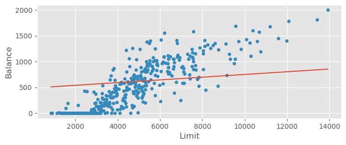
Even though the model does not produce negative values anymore, it’s bias is now too strong! The visible trend cannot be fitted. This model should definitely not be used.
Exercise 3: Multiple Linear Regression on Insurance Data
In this exercise, we are going to look at a sample insurance dataset that you can find in insurance.csv. The goal is to use the set of predictors provided in the data to predict the yearly charges in USD for clients to get an estimate of the overall reserve budget.
a)
Load the dataset with Pandas and get an overview over the nature of the different predictors that are provided. For a first analysis, we will use the predictors age, bmi and smoker for an estimation of the total charges. To this end, perform an exploratory data analysis and plot age and bmi against charges in two separate plots. Since smoker is a categorical variable, use it to color your observations (e.g. in seaborn with the hue parameter).
insurance_data = pd.read_csv("insurance.csv")
insurance_data.head()sns.scatterplot( data=insurance_data, x="age", y="charges", hue="smoker" )<Axes: xlabel='age', ylabel='charges'>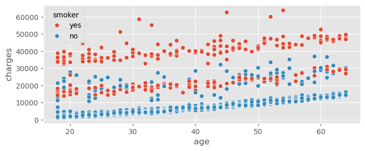
sns.scatterplot( data=insurance_data, x="bmi", y="charges", hue="smoker" )<Axes: xlabel='bmi', ylabel='charges'>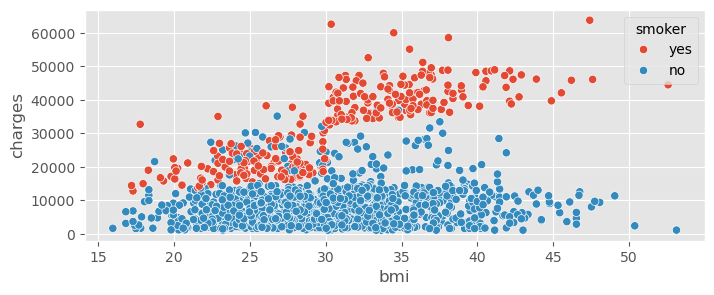
Smoker is clearly a very important variable!
b)
Fit a multiple Bayesian linear regression model with Bambi that predicts charges from age, bmi and smoker. Summarize the 95% HDIs for all involved parameters and give an interpretation for the role of each parameter in the prediction. Are all parameters significant in the Bayesian sense? Compute Bayesian RMSE and to quantify the performance of the model.
insurance_model1 = bmb.Model("charges ~ age + bmi + smoker", data=insurance_data, family="gaussian")
insurance_trace1 = insurance_model1.fit(draws=2000, tune=2000)
pm.summary( insurance_trace1, hdi_prob=0.95 )All parameters are significant at the 95% level (no HDI includes zero). The model can be interpreted as follows: Each year of age results in a mean of 260 USD of additional charges, a BMI increase of 1 results in a mean of additional 322 USD of charges and smokers have on average 23’800 USD more insurance charges than non-smokers!
insurance_model1.predict(insurance_trace1, kind="response")
ypred = az.extract( insurance_trace1.posterior_predictive ).charges.values.T
ytrue = insurance_data.charges.values
RMSE:
np.sqrt( np.mean( (ypred - ytrue)**2 ) )np.float64(8621.337788653796)Our predictions will typically be away from the ground truth by ± 8600 USD!
:
pm.r2_score( ytrue, ypred )r2 0.663960
r2_std 0.010121
dtype: float64There is still a lot of variance to be explained!
c)
Fit a model with all the available predictors. Do all predictors significantly contribute to the predictions of the model? Compute Bayesian RMSE and to quantify the performance of the model. Which model would you rather use, the previous model including only age, bmi and smoker as predictors or the more complex current one?
insurance_data.head()insurance_model2 = bmb.Model("charges ~ age + sex + bmi + children + smoker + region", data=insurance_data, family="gaussian")
insurance_trace2 = insurance_model2.fit(draws=2000, tune=2000)
pm.summary( insurance_trace2, hdi_prob=0.95 )Sex and region[northwest] do not contribute significantly at the 95% level (HDIs include zero).
Performance metrics:
insurance_model2.predict(insurance_trace2, kind="response")
ypred = az.extract( insurance_trace2.posterior_predictive ).charges.values.T
ytrue = insurance_data.charges.values
RMSE:
np.sqrt( np.mean( (ypred - ytrue)**2 ) )np.float64(8578.626184138278):
pm.r2_score( ytrue, ypred )r2 0.666538
r2_std 0.010132
dtype: float64The improvement in terms of metrics is marginal. Rather use the more simple model from b) for this data!
d)
Could your more complex model get better with more data? Compute epistemic and aleatoric variance of the predictive distribution on your dataset using predict() and setting data = insurance_data.
Hint: The rest is like in Exercise 1.
Compute model predictions:
pred = insurance_model2.predict( insurance_trace2, kind="response", data=insurance_data, inplace=False )Compute different uncertainties (see lecture):
var_e = pred.posterior.mu.var().values
np.sqrt( var_e )np.float64(10499.037071488348)var_p = pred.posterior_predictive.charges.var().values
np.sqrt( var_p )np.float64(12125.139005403647)var_a = var_p - var_e
np.sqrt( var_a )np.float64(6065.411484134803)var_e / var_p, var_a / var_p(np.float64(0.749765557528311), np.float64(0.25023444247168897))There is a significant part of epistemic uncertainty! With more data we might thus also be able to use a model with more predictors (emphasis on might).
e)
It is often said that there is an aggravating effect when an individual is both overweight and a smoker, with even bigger impacts than just the sum of the two on personal health. You want to verify this on the given dataset by adding an interaction term between bmi and smoker. Fit a model and report and interpret your results with pm.summary(). Did your prediction performance in terms of increase?
insurance_model3 = bmb.Model("charges ~ age + bmi + smoker + bmi:smoker", data=insurance_data, family="gaussian")
insurance_trace3 = insurance_model3.fit(draws=2000, tune=2000)
pm.summary( insurance_trace3, hdi_prob=0.95 )The interaction term is significant (and large), let’s keep it if the predicitive performance increases as well:
insurance_model3.predict(insurance_trace3, kind="response")
ypred = az.extract( insurance_trace3.posterior_predictive ).charges.values.T
ytrue = insurance_data.charges.values
pm.r2_score( ytrue, ypred )
r2 0.752790
r2_std 0.008084
dtype: float64A very significant improvement by almost 9% in explained variance! This is a clear indicator that this interaction term cannot be neglected when doing predictions.
f)
Go back to your initial plots in a). Is evidence for the significant interaction between overweight and smoking visible in one of the plots?
sns.scatterplot( data=insurance_data, x="bmi", y="charges", hue="smoker" )<Axes: xlabel='bmi', ylabel='charges'>The dependence of charges on BMI is much steeper if the client is a smoker!
Exercise 4: Multiple Linear Regression on Advertisement Data
In this exercise you will perform multiple linear regression on the advertisement dataset introduced by the famous book Introduction to Statistical Learning. It contains data of an advertisement campaign with the budget used for TV, radio and newspaper ads in 1000 USD against the number of units that were sold (in thousands).
a)
Load the dataset with Pandas and get an overview over the different predictors that are provided. Create some exploratory plots to guess which variables will probably be related to the sales variable.
adv_data = pd.read_csv("advertising.csv")
adv_data.head()sns.scatterplot( data=adv_data, x="TV", y="sales" )<Axes: xlabel='TV', ylabel='sales'>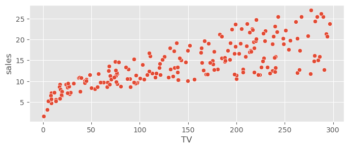
sns.scatterplot( data=adv_data, x="radio", y="sales" )<Axes: xlabel='radio', ylabel='sales'>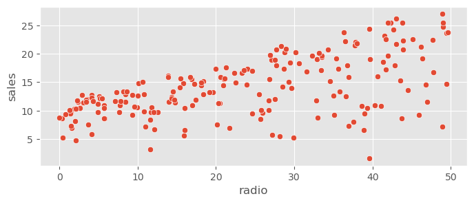
sns.scatterplot( data=adv_data, x="newspaper", y="sales" )<Axes: xlabel='newspaper', ylabel='sales'>
Expect contributions by radio and TV, probably not by newspaper.
b)
Fit a multiple linear regression model including all the available predictors. Which contribute significantly to the model? What is your interpretation of the coefficients?
adv_model1 = bmb.Model("sales ~ TV + radio + newspaper", data=adv_data, family="gaussian")
adv_trace1 = adv_model1.fit(draws=2000, tune=2000)
pm.summary( adv_trace1, hdi_prob=0.95 )The 95% HDI for newspaper includes zero, thus newspaper does not contribute significantly at the 95% level. For each 1000 USD spent on TV ads, 46 more units are sold (43-49 in 95% HDI), for each 1000 USD spent on radio ads, 189 more units are sold (172-205 in 95% HDI).
c)
Compute predictive RMSE and score. Is this a good model? Give an interpretation in particular of RMSE.
adv_model1.predict(adv_trace1, kind="response")
ypred = az.extract( adv_trace1.posterior_predictive ).sales.values.T
ytrue = adv_data.sales.values
RMSE:
rmse = np.sqrt( np.mean( (ypred - ytrue)**2 ) )
rmsenp.float64(2.392592625451304)rmse / np.mean(adv_data.sales)np.float64(0.17062525408816573)Our predictions will typically be away from the true value by ± 2400 sold units, this is about 20% of the units being typically sold. For the advertisement business I wouldn’t expect much more..
:
pm.r2_score( ytrue, ypred )r2 0.826892
r2_std 0.015734
dtype: float64d)
Refit your model without newspaper. Do RMSE and change significantly?
adv_model2 = bmb.Model("sales ~ TV + radio", data=adv_data, family="gaussian")
adv_trace2 = adv_model2.fit(draws=2000, tune=2000)
pm.summary( adv_trace2, hdi_prob=0.95 )adv_model2.predict(adv_trace2, kind="response")
ypred = az.extract( adv_trace2.posterior_predictive ).sales.values.T
ytrue = adv_data.sales.valuesRMSE:
np.sqrt( np.mean( (ypred - ytrue)**2 ) )np.float64(2.386114969682464):
pm.r2_score( ytrue, ypred )r2 0.827571
r2_std 0.015798
dtype: float64No significant changes in RMSE or .
e)
There might be synergy or redundancy between TV and radio advertisement budget: either viewers who get the ad through both channels are even more inclined to buy the product (synergy) or it is enough that they hear it through one channel and the other one is an unnecessary repetition (redundancy), or something in-between of course. Introduce an interaction between TV and radio and interpret your results. Is the interaction term significant? Can we observe a synergy or a redundancy? How does the predictive performance change?
adv_model3 = bmb.Model("sales ~ TV + radio + TV:radio", data=adv_data, family="gaussian")
adv_trace3 = adv_model3.fit(draws=2000, tune=2000)
pm.summary( adv_trace3, hdi_prob=0.95 )The interaction term is significant and positive - meaning that if TV and radio are high, the amount of sales is even higher (synergy).
Predictive performance:
adv_model3.predict(adv_trace3, kind="response")
ypred = az.extract( adv_trace3.posterior_predictive ).sales.values.T
ytrue = adv_data.sales.values
RMSE:
rmse = np.sqrt( np.mean( (ypred - ytrue)**2 ) )
rmsenp.float64(1.3383383616612556)rmse / adv_data.sales.mean()np.float64(0.09544220799866326)Our predictions will now typically be away from the true value by only ± 1300 sold units! this is about 10% of the units being typically sold! This is good..
:
pm.r2_score( ytrue, ypred )r2 0.938312
r2_std 0.006006
dtype: float64A large part of the variance is now explained.
f)
You might have noticed in the exploratory analysis performed in part a) that you are rather in a heteroscedastic than a homescedastic setting, where variance is not constant anymore but depends on the value of the predictor. To alleviate this, model the logarithm of sales instead of just sales. Show using scatter plots that this is a reasonable approach and compare the performance of your resulting model (including interactions) with your model from d).
adv_data['logsales'] = np.log( adv_data.sales )
adv_data.head()sns.scatterplot( data=adv_data, x="TV", y="logsales", )<Axes: xlabel='TV', ylabel='logsales'>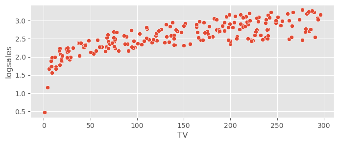
sns.scatterplot( data=adv_data, x="radio", y="logsales" )<Axes: xlabel='radio', ylabel='logsales'>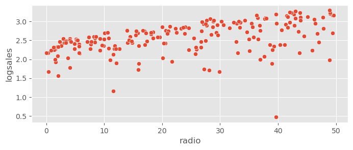
sns.scatterplot( data=adv_data, x="newspaper", y="logsales" )<Axes: xlabel='newspaper', ylabel='logsales'>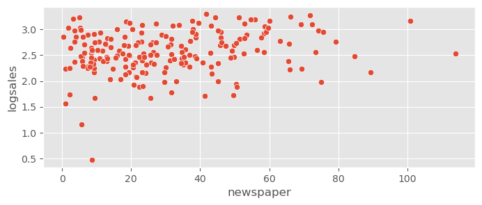
The variance is now more constant along the predictors, however the residuals look a bit more skewed now. Let’s check how this works!
adv_model4 = bmb.Model("logsales ~ TV + radio + TV:radio", data=adv_data, family="gaussian")
adv_trace4 = adv_model4.fit(draws=2000, tune=2000)
pm.summary( adv_trace4, hdi_prob=0.95 )Predictive performance:
adv_model4.predict(adv_trace4, kind="response")
ypred = np.exp( az.extract( adv_trace4.posterior_predictive ).logsales.values.T )
ytrue = adv_data.sales.values
RMSE:
rmse = np.sqrt( np.mean( (ypred - ytrue)**2 ) )
rmsenp.float64(3.2639485089464157)rmse / adv_data.sales.mean()np.float64(0.23276509245472743):
pm.r2_score( ytrue, ypred )r2 0.796211
r2_std 0.017985
dtype: float64The model performs much worse. Probably because we violated the assumption of normally distributed residuals.
Exercise 5: Robust Linear Regression
In this exercise, you will model body fat from BMI (data in bodyfat.csv) as done in the lecture, however including the real outliers in the dataset.
a)
Load the dataset with Pandas, create a scatter plot of BMI against BodyFat and convince your self of the presence of outliers that might influence the coefficients of linear models.
bodyfat_data = pd.read_csv("bodyfat.csv")
bodyfat_data.head()sns.scatterplot( bodyfat_data, x="BMI", y="BodyFat" )<Axes: xlabel='BMI', ylabel='BodyFat'>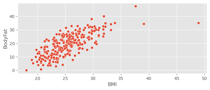
b)
Fit a simple linear regression model with normal likelihood with Bambi and assess its predictive performance in terms of RMSE and . In addition, plot the regression model with bmb.interpret.plot_predictions().
bodyfat_model1 = bmb.Model("BodyFat ~ BMI", data=bodyfat_data, family="gaussian")
bodyfat_trace1 = bodyfat_model1.fit(draws=2000, tune=2000)
pm.summary( bodyfat_trace1, hdi_prob=0.95 )Plot:
bodyfat_data.plot.scatter( x="BMI", y="BodyFat" )
bmb.interpret.plot_predictions( bodyfat_model1, bodyfat_trace1, "BMI", prob=0.95, ax=plt.gca() )
(<Figure size 800x300 with 1 Axes>,
array([<Axes: xlabel='BMI', ylabel='BodyFat'>], dtype=object))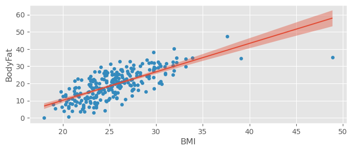
Predictive performance:
bodyfat_model1.predict(bodyfat_trace1, kind="response")
ypred = az.extract( bodyfat_trace1.posterior_predictive ).BodyFat.values.T
ytrue = bodyfat_data.BodyFat.values
RMSE:
np.sqrt( np.mean( (ypred - ytrue)**2 ) )np.float64(8.151465963173502)Our predictions will now typically be away from the true value by around ± 8%.
:
pm.r2_score( ytrue, ypred )r2 0.513199
r2_std 0.027314
dtype: float64There are better values in the world..
c)
As an alternative, fit a robust model that uses a Student’s t distribution as likelihood instead of a normal distribution (see exercises in week 5 for insights into Student’s t distribution). You may do this with Bambi by choosing family="t" instead of family="gaussian". Do the non-robust and the robust model differ significantly? Compare RMSE and and plot both models in the same plot with bmb.interpret.plot_predictions(). Which model would you use at the end?
bodyfat_model2 = bmb.Model("BodyFat ~ BMI", data=bodyfat_data, family="t")
bodyfat_trace2 = bodyfat_model2.fit(draws=2000, tune=2000)
pm.summary( bodyfat_trace2, hdi_prob=0.95 )Plot:
bodyfat_data.plot.scatter( x="BMI", y="BodyFat" )
bmb.interpret.plot_predictions( bodyfat_model1, bodyfat_trace1, "BMI", prob=0.95, ax=plt.gca() )
bmb.interpret.plot_predictions( bodyfat_model2, bodyfat_trace2, "BMI", prob=0.95, ax=plt.gca() )
(<Figure size 800x300 with 1 Axes>,
array([<Axes: xlabel='BMI', ylabel='BodyFat'>], dtype=object))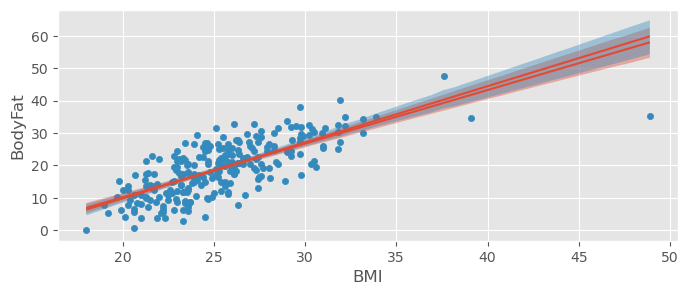
Predictive performance:
bodyfat_model2.predict(bodyfat_trace2, kind="response")
ypred = az.extract( bodyfat_trace2.posterior_predictive ).BodyFat.values.T
ytrue = bodyfat_data.BodyFat.values
RMSE:
np.sqrt( np.mean( (ypred - ytrue)**2 ) )np.float64(8.182406471636726)Our predictions will now typically be away from the true value by around .
:
pm.r2_score( ytrue, ypred )r2 0.524749
r2_std 0.027579
dtype: float64Only very slight improvement! Probably better prefer the simpler model.
d)
As an addition model selection tool, you consider computing ELPDs for both models and to compare them (see week 5). Compute the log-likelihood for both model traces with pm.compute_log_likelihood() (in the context of the underlying PyMC model that can be accessed through backend.model) and then use pm.compare() and pm.plot_compare(). Which do you trust more in this case, RMSE and or ELPD?
Compute log likelihoods:
with bodyfat_model1.backend.model:
    pm.compute_log_likelihood( bodyfat_trace1 )

with bodyfat_model2.backend.model:
pm.compute_log_likelihood( bodyfat_trace2 )Compare ELPDs:
compare_dict = {
    'Normal model': bodyfat_trace1,
    'Robust model': bodyfat_trace2
}
comp = pm.compare( compare_dict )
comppm.plot_compare( comp )<Axes: title={'center': 'Model comparison\nhigher is better'}, xlabel='elpd_loo (log)', ylabel='ranked models'>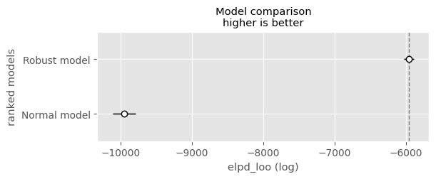
There seems to a big difference in terms of predictive performance. However both loo estimates produced warnings and our predictive performance estimates say otherwise. Personally, I would trust more in RMSE and here.
e)
Just for fun: Fit a robust multiple linear regression model with all variables (except Density that is used to compute BodyFat) and check whether it is an improvement on the models in b) and c) in terms of RMSE and . Check the posterior distribution of . Would you at the end rather use a normal or a Student’s t likelihood?
bodyfat_data.head()bodyfat_model3 = bmb.Model(
"BodyFat ~ Age + Weight + Height + Neck + Chest + Abdomen + Hip + Thigh + Knee + Ankle + Biceps + Forearm + Wrist + BMI",
data=bodyfat_data,
family="t"
)
bodyfat_trace3 = bodyfat_model3.fit(draws=2000, tune=2000)
pm.summary( bodyfat_trace3, hdi_prob=0.95 )The uncertainty on is still quite large! Since it is large (mean of 33), probably a normal likelihood could be preferred. The following variables do not seem to be significant at to 95% level: Neck, Chest, Thigh, Knee, Ankle, Biceps, Forearm. It might make sense to refit a model without them.
Predictions:
bodyfat_model3.predict(bodyfat_trace3, kind="response")
ypred = az.extract( bodyfat_trace3.posterior_predictive ).BodyFat.values.T
ytrue = bodyfat_data.BodyFat.values
RMSE:
np.sqrt( np.mean( (ypred - ytrue)**2 ) )np.float64(6.068379228018641)Our predictions will now typically be away from the true value by around , this is 25% better!
:
pm.r2_score( ytrue, ypred )r2 0.662684
r2_std 0.023387
dtype: float64Quite a bit more variance explained!
Exercise 6: Leaking Satellite Fuel Tank
You work for the European Space Agency in the maintenance team for a satellite. Next to scientific data, the satellite sends back a host of maintenance data, among other things the fuel level of its thrusters that are needed to keep it on the designed orbit. Since sending satellite data down to Earth is expensive (antenna network distributed over the Earth) and a large part of the bandwidth is reserved for scientific data and redundancy, you get only one fuel level measurement per day.
Three days ago you have discovered that the fuel tank level has decreased by a larger amount than usual. You suspect that the satellite has been hit by space debris that has produced a hole in the fuel tank. The goal of this exercise is to compute the remaining time in the satellite mission, before the thrusters fail by lack of fuel and the satellite will leave its carefully calibrated orbit.
a)
Load the dataset from fuel_data.csv. It contains the time in days (starting from zero), the tank level in milligrams and the suspected state of the fuel tank (nominal/leaking). Plot the tank level against the time and verify that the point in time where the tank level decreases more quickly is visible (at ).
fuel_data = pd.read_csv("fuel_data.csv")
fuel_dataPlot:
sns.lineplot( data=fuel_data, x="t", y="tank_level", c="black" )
sns.scatterplot( data=fuel_data, x="t", y="tank_level", hue="state", s=50 )
<Axes: xlabel='t', ylabel='tank_level'>
b)
First you fit a model to the nominal data points with the yet intact fuel tank to guess the regular rate of fuel consumption in mg. To this end, fit a linear regression model to and guess a 95% HDI of .
Because there is prior information available from your engineering team, you decide to choose your own priors instead of letting Bambi choose weak default priors:
Bambi chooses for intercept not the value at , but the value in the center of the data distribution. In this case, the center falls between 9 and 10, so you choose as intercept . The engineers in your project team say that there is an uncertainty of mg in the tank level.
For fuel rate, your engineering team says that the thrusters consume at around per day, possibly also something between and . Use PreliZ to devise an appropriate normal prior. Hint: Make sure that the rate is negative (decrease).
Pass your priors to bambi and fit a model to the first 20 data points (). Visualize your model predictions with bmb.interpret.plot_predictions() with pps=True and estimate a 95% HDI for the regular fuel consumption rate .
Prior for intercept:
y0 = (fuel_data.tank_level[9]+fuel_data.tank_level[10])/2
pz.Normal(y0, 0.2).plot_pdf()
<Axes: >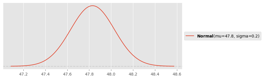
Prior for regular fuel decrease:
pz.Normal(-0.04, 0.01).plot_pdf()<Axes: >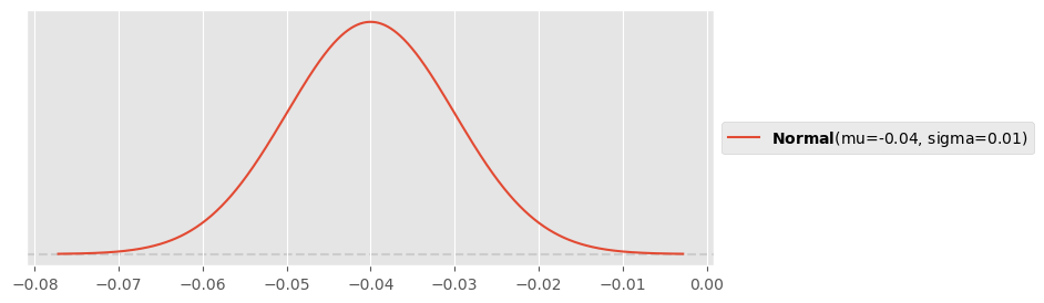
Fit model:
priors = {
    "Intercept": bmb.Prior("Normal", mu=y0, sigma=0.2),
    "t": bmb.Prior("Normal", mu=-0.04, sigma=0.01),
}
normal_tank_model = bmb.Model("tank_level ~ t", data=fuel_data[fuel_data.t <= 19], priors=priors, family="gaussian")
normal_tank_trace = normal_tank_model.fit(draws=2000, tune=2000)fuel_data.plot( x="t", y="tank_level", marker="o", c="blue" )
bmb.interpret.plot_predictions( normal_tank_model, normal_tank_trace, "t", prob=0.95, pps=True, ax=plt.gca() )(<Figure size 800x300 with 1 Axes>,
array([<Axes: xlabel='t', ylabel='tank_level'>], dtype=object))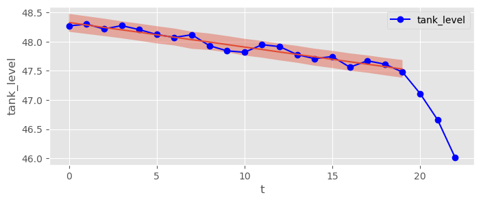
pm.summary( normal_tank_trace, hdi_prob=0.95 )Typical fuel consumption between 37 and 47 per day (95% HDI, results may vary slightly for different simulations).
c)
Now fit a model to the data points where you suspect the leak (). This time let Bambi choose default priors for you. Visualize your model predictions again with bmb.interpret.plot_predictions() with pps=True and estimate a 95% HDI for the leaking fuel consumption rate .
fuel_data[fuel_data.t>=19]leaking_tank_model = bmb.Model("tank_level ~ t", data=fuel_data[fuel_data.t>=19], family="gaussian")
leaking_tank_trace = leaking_tank_model.fit(draws=2000, tune=2000)fuel_data.plot( x="t", y="tank_level", marker="o", c="blue" )
bmb.interpret.plot_predictions( leaking_tank_model, leaking_tank_trace, "t", prob=0.95, ax=plt.gca() )(<Figure size 800x300 with 1 Axes>,
array([<Axes: xlabel='t', ylabel='tank_level'>], dtype=object))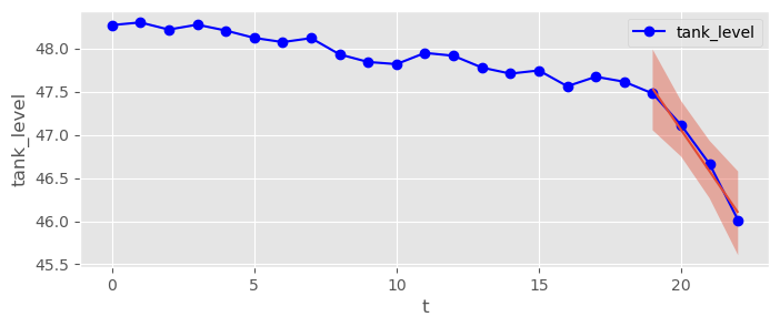
pm.summary( leaking_tank_trace )fuel loss between 228 and 697 g per day! (results may vary from simulation to simulation, will get better with more data)
d)
Mission control asks you how long they can expect the satellite mission to continue, i.e. how many days the mission can last until the fuel tank is empty. Use the 95% HDI on to give an estimate.
t0 = fuel_data.tank_level[22] / np.abs( pm.hdi( leaking_tank_trace.posterior.t, 0.95 ) )
t0Between 63 and 232 days with a belief of 95%, however this is probably quite uncertain (especially if you re-run the simulation). You’ll know more with more data!
Let us plot the distribution to better understand our uncertainty:
t0_values = -fuel_data.tank_level[22] / leaking_tank_trace.posterior.t.values.flatten()
plt.hist( t0_values.clip(0, 300), bins=20 );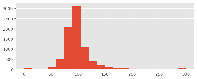
(a few strong outliers - interesting exercise: find a good prior for to make them disappear)