Bayesian Linear Regression
Simple linear regression
We start with a single predictor and a continuous response .
The deterministic regression line is
with intercept and slope .
To make this into a probabilistic model, we add a noise term:
Equivalently, the likelihood for each observation is
In vector–matrix form, with design matrix
the model is
Likelihood and ordinary least squares (OLS)
Under the normal likelihood
the log-likelihood (up to additive constants) is
Maximizing this log-likelihood w.r.t. (for fixed ) is equivalent to minimizing the sum of squared residuals:
In matrix form, the OLS solution has a closed form:
provided is invertible.
OLS is the maximum likelihood estimator for under the normal linear model with constant variance .
Bayesian linear regression
In the Bayesian view, the parameters are random variables with a prior distribution.
A common prior choice (conceptually) is:
Regression coefficients:
Noise scale:
Given the data , the posterior over parameters is
Using Bayes’ theorem explicitly,
For conjugate priors (normal–inverse-gamma), the posterior has an analytic form; in practice we often let PyMC/Bambi do the MCMC sampling from .
Posterior predictive distribution for regression
For a new input , the model implies
The posterior predictive distribution, which averages over uncertainty in , is
In practice, with posterior samples , we approximate this by simulation:
For each posterior draw ,
The sample approximates .
The posterior predictive distribution combines:
Aleatoric uncertainty: the inherent noise in ,
Epistemic uncertainty: uncertainty about due to finite data.
Epistemic vs aleatoric uncertainty in regression
In the linear model
we distinguish:
Aleatoric uncertainty: variability in even if were known exactly. In this model, for a fixed , this is just .
Epistemic uncertainty: additional variability in predictions due to uncertainty in as captured by the posterior .
For the posterior predictive variance at a given , the law of total variance gives
where .
The first term corresponds to aleatoric variance (expected ).
The second term corresponds to epistemic variance (spread of the regression line due to parameter uncertainty).
With many data points covering a range of , the epistemic term often becomes small near the data but remains large when extrapolating far away from observed values.
Gaussian linear regression
import numpy as np
import matplotlib.pyplot as plt
from ipywidgets import interact, IntSlider, FloatSlider, Checkbox

plt.rcParams["figure.figsize"] = (4, 4)
Linear regression is perhaps the most frequently used technique in applied statistics for modelling the relationship between set of a predictor variables and a response variable . More formally, let be a design matrix and let be the response variables collected into a single vector, then the linear regression model is given by
where is the regression weights and is the observation noise vector.
Assuming isotropic Gaussian noise and imposing a multivariate Gaussian prior on gives rise to the following joint distribution
In this notebook, we will use the following simple model as running example:
That is, the parameters are , where and are the slope and intercept of the line, respectively. Furthermore, we will assume , , and .
We will use the following dataset with data points
Source
# hyperparameters of the prior
m = np.zeros((2, 1))
S = 1.0*np.identity(2)

# noise variance
sigma2 = 2

# data
N = 8
x = np.array([1.764, 0.4, 0.979, 2.241, 1.868, -0.977,  0.95, -0.151])[:, None]
y = np.array([-0.464, 2.024, 3.191, 2.812, 6.512, -3.022, 1.99, 0.009])[:, None]

# plot
plt.plot(x, y, 'k.', label='Data', markersize=12)
plt.xlabel('Predictor Variable x')
plt.ylabel('Response y')
plt.legend()
plt.xlim((-3, 3))
plt.ylim((-6, 6))
plt.grid()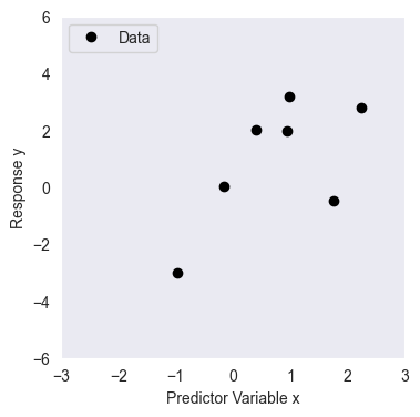
The prior, likelihood and posterior
This section illustrates the basic building blocks of the linear model.
Reference: Rasmussen and Williams, Section 2.1, for the derivation of these functions (http://
The multivariate Gaussian density function
The multivariate Gaussian density function, implemented using numpy.
def mvn_pdf(x, mu, Sigma, log=True):
    """ Returns the density of a multivariate Gaussian distribution
    with mean mu and covariace Sigma at point x

    Arguments:
    x     -- (Dx1) evaluation point
    mu    -- (Dx1) mean vector
    Sigma -- (DxD) covariance matrix
    log   -- (bool) if true, return log density. If false, return the density. (default=True)

    Returns:
    (scalar) density
    """
    D = len(mu)
    Sigma = Sigma + 1e-10 * np.identity(D)
    L = np.linalg.cholesky(Sigma)
    v = np.linalg.solve(L, x-mu)
    const_term = -0.5 * D * np.log(2 * np.pi)
    det_term = -0.5 * 2 * np.sum(np.log(np.diag(L)))
    quad_term = -0.5 * np.sum(v ** 2)
    if log:
        return const_term + det_term + quad_term
    else:
        return np.exp(const_term + det_term + quad_term)
Computes the (log-)density of a multivariate Gaussian using a numerically stable Cholesky decomposition of the covariance matrix.
Adds a small diagonal jitter to to ensure positive definiteness and avoid numerical issues during factorization.
Uses the Cholesky factor to efficiently solve , which is required to compute the quadratic form .
Combines the constant term, log-determinant term (computed from ), and quadratic term to return either the log-density or the density.
Source
from scipy.stats import multivariate_normal
import gaussian_linear_regression as glr

x_test = np.array([1,1])
print("Scipy multivariate_normal model")
pdf = multivariate_normal.pdf(x_test, mean=m.flatten(), cov=S)
print("The pdf of [1,1] is", pdf)
logpdf = multivariate_normal.logpdf(x_test, mean=m.flatten(), cov=S)
print("The logpdf of [1,1] is", logpdf)

x_test = np.array([1,1]).reshape(2,1)
print("\nOwn mvn_pdf")
pdf = glr.mvn_pdf(x_test, mu=m, Sigma=S, log=False)
print("The pdf of [1,1] is", pdf)
logpdf = glr.mvn_pdf(x_test, mu=m, Sigma=S, log=True)
print("The logpdf of [1,1] is", logpdf)
Scipy multivariate_normal model
The pdf of [1,1] is 0.05854983152431917
The logpdf of [1,1] is -2.8378770664093453
Own mvn_pdf
The pdf of [1,1] is 0.05854983152431917
The logpdf of [1,1] is -2.8378770664093453
The Log density functions
The Log density of the (i) prior, (ii) likelihood, and (iii) posterior (likelihood times prior), implemented using the mvn_pdf function.
def log_prior(a, b, m, S):
    """ returns the log density of the prior at the points (a,b) given m and S

    Arguments:
    a    -- (scalar) slope parameter
    b    -- (scalar) intercept parameter
    m    -- (2x1) The prior mean
    S    -- (2x2) The prior covariance

    Returns
    (scalar) log density for the pair (a,b)

    """
    return mvn_pdf(np.array([a,b])[:, None], m, S, log=True)

def log_likelihood(x, y, a, b, sigma2):
    """ returns the log-likelihood for the data (x,y) given the parameters (a,b)

    Arguments:
    x    -- (Nx1) vector of inputs
    y    -- (Nx1) vector of responses
    a    -- slope parameter
    b    -- intercept parameter

    Returns:
    (scalar) log likelihood of (x,y)
    """
    log_npdf = lambda x, m, v: -0.5 * np.log(2* np.pi * v) - 0.5 * (x - m)**2/v
    return np.sum(log_npdf(y, predict(x,a,b), sigma2))


def log_posterior(x, y, a, b, m, S, sigma2):
    """Returns the log posterior at (a,b), given the data (x,y) and the prior parameters (m, S).

    Arguments:
    x    -- (Nx1) vector of inputs
    y    -- (Nx1) vector of responses
    a    -- slope parameter
    b    -- intercept parameter
    m    -- (2x1) prior mean of (a, b)
    S    -- (2x2) prior covariance of (a, b)
    sigma2 -- (scalar) noise variance

    Returns:
    (scalar) log posterior at (a, b)
    """
    return log_prior(a, b, m, S) + log_likelihood(x, y, a, b, sigma2)

def compute_posterior(x, y, m, S, sigma2):
    """ return the posterior mean and covariance of w given (x,y)
    and hyperparameters m, S and sigma2

    Arguments:
    x      -- (Nx1) vector of inputs
    y      -- (Nx1) vector of responses
    m      -- (Dx1) prior mean
    S      -- (DxD) prior covariance
    sigma2 -- (scalar) noise variance

    Returns:
    mu     -- (Dx1) posterior mean
    Sigma  -- (DxD) posterior covariance

    """
    import scipy as sc
    Sinv = np.linalg.inv(S)
    X = design_matrix(x)
    Sigmainv = Sinv + np.dot(X.T, X)/sigma2
    L = sc.linalg.cho_factor(Sigmainv)
    scaled_mu = np.divide(np.dot(X.T, y), sigma2).reshape(-1, 1) + np.linalg.solve(S, m)
    mu = sc.linalg.cho_solve(L, scaled_mu)
    Sigma = sc.linalg.cho_solve(L, np.identity(len(m)))

    assert mu.shape == m.shape
    assert S.shape == Sigma.shape

    return mu, Sigma
The Visualization
Visualization of the prior density, the likelihood and the posterior as a function of and .
def plot_prior_density(m, S, a, b):
    A_array, B_array = np.meshgrid(a, b)
    Z = np.array([log_prior(ai, bi, m, S) for (ai, bi) in zip(A_array.ravel(), B_array.ravel())])
    Z = Z.reshape((len(a), len(b)))
    plt.contour(a, b, log_to_density(Z), cmap='plasma')
    plt.xlabel('slope')
    plt.ylabel('intercept')
    plt.gca().set_aspect('equal', adjustable='box')

def plot_likelihood(x, y, sigma2, a, b):
    A_array, B_array = np.meshgrid(a, b)
    Z = np.array([log_likelihood(x, y, ai, bi, sigma2) for (ai, bi) in zip(A_array.ravel(), B_array.ravel())])
    Z = Z.reshape((len(a), len(b)))
    plt.contour(a, b, log_to_density(Z), 10, cmap='plasma')
    plt.xlabel('slope')
    plt.ylabel('intercept')
    plt.gca().set_aspect('equal', adjustable='box')

def plot_posterior_density(x, y, m, S, sigma2, a, b):
    A_array, B_array = np.meshgrid(a, b)
    Z = np.array([log_posterior(x, y, ai, bi, m, S, sigma2) for (ai, bi) in zip(A_array.ravel(), B_array.ravel())])
    Z = Z.reshape((len(a), len(b)))
    plt.contour(a, b, log_to_density(Z), 10, cmap='plasma')
    plt.xlabel('slope')
    plt.ylabel('intercept')
    plt.gca().set_aspect('equal', adjustable='box')

def log_to_density(Z):
    Z = Z - np.max(Z)
    Z = np.exp(Z)
    return Z/np.sum(Z)

def plot_posterior_credibility_region(x, y, m, S, sigma2, xp):
    mu, Sigma = compute_posterior(x, y, m, S, sigma2)
    mu_f, var_f = compute_f_posterior(xp, mu, Sigma)

    std_f = np.sqrt(var_f)
    mu_f = mu_f.reshape(-1)
    std_f = std_f.reshape(-1)

    plt.figure(figsize=(12, 4))
    plt.plot(x, y, 'k.', markersize=12, label='observations')
    plt.plot(xp, mu_f, 'b', label='mean prediction')
    plt.fill_between(xp, mu_f - 2 * std_f, mu_f + 2 * std_f, alpha=0.2, color='r', label='Posterior credibility region')
    plt.legend()
    plt.grid()

def plot_predictive_region(x, y, m, S, sigma2, xp):
    mu, Sigma = compute_posterior(x, y, m, S, sigma2)
    mu_f, var_f = compute_f_posterior(xp, mu, Sigma)
    mu_f = mu_f.reshape(-1)

    var_y = var_f + sigma2
    std_y = np.sqrt(var_y)
    std_y = std_y.reshape(-1)

    plt.plot(x, y, 'k.', markersize=12, label='observations')
    plt.plot(xp, mu_f, 'b', label='mean prediction')
    plt.fill_between(
        xp,
        mu_f - 2 * std_y,
        mu_f + 2 * std_y,
        alpha=0.2,
        color='r',
        label='Predictive 95% region'
    )
    plt.legend()
    plt.grid()

def rmse(mu_f, y):
    return np.sqrt(np.mean((y - mu_f)**2))

def mae(mu_f, y):
    return np.mean(np.abs(y - mu_f))

def r2(mu_f, y):
    return 1 - np.mean((y - mu_f)**2) / np.var(y)
Source
import gaussian_linear_regression as glr

a = np.linspace(-3,3,100)
b = np.linspace(-3,3,100)

# plot
plt.figure(figsize=(18,6))
plt.subplot(1, 3, 1)
glr.plot_prior_density(m, S, a, b)
plt.title('Prior')
plt.grid()

plt.subplot(1, 3, 2)
glr.plot_likelihood(x, y, sigma2, a, b)
plt.title('Likelihood')
plt.grid()

plt.subplot(1, 3, 3)
glr.plot_posterior_density(x, y, m, S, sigma2, a, b)
plt.title('Posterior')
plt.grid()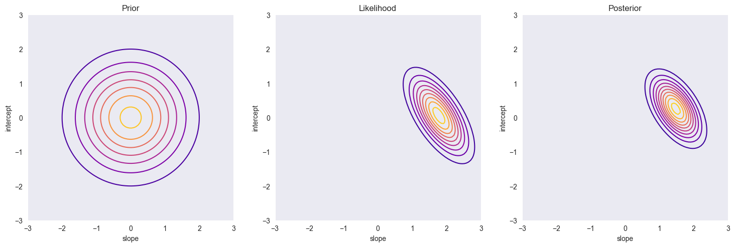
Analytical expression of the posterior distribution
Derivation of the posterior yields:
Reference: Rasmussen and Williams, Section 2.1.1, for the derivation of these functions (http://
The Implementation
Implementation of the function for computing the analytical posterior distribution.
def compute_posterior(x, y, m, S, sigma2):
    """ return the posterior mean and covariance of w given (x,y)
    and hyperparameters m, S and sigma2

    Arguments:
    x      -- (Nx1) vector of inputs
    y      -- (Nx1) vector of responses
    m      -- (Dx1) prior mean
    S      -- (DxD) prior covariance
    sigma2 -- (scalar) noise variance

    Returns:
    mu     -- (Dx1) posterior mean
    Sigma  -- (DxD) posterior covariance

    """
    import scipy as sc
    Sinv = np.linalg.inv(S)
    X = design_matrix(x)
    Sigmainv = Sinv + np.dot(X.T, X)/sigma2
    L = sc.linalg.cho_factor(Sigmainv)
    scaled_mu = np.divide(np.dot(X.T, y), sigma2).reshape(-1, 1) + np.linalg.solve(S, m)
    mu = sc.linalg.cho_solve(L, scaled_mu)
    Sigma = sc.linalg.cho_solve(L, np.identity(len(m)))

    assert mu.shape == m.shape
    assert S.shape == Sigma.shape

    return mu, Sigma

def design_matrix(x):
    """ returns the design matrix for a vector of input values x

    Arguments:
    x    -- (Nx1) vector of inputs

    Returns:
    (Nx2) design matrix

    """
    X = np.column_stack((x, np.ones(len(x))))
    return X
Computes the inverse of the posterior covariance matrix using the inverse of the prior covariance
Sinv = np.linalg.inv(S)and the design matrixX = design_matrix(x).Forms the Cholesky factorization of the inverse of the inverse posterior covariance matrix using
sc.linalg.cho_factor(Sigmainv), enabling stable and efficient solutions for both the posterior mean and covariance without explicitly inverting matrices.Computes the scaled right-hand side using
np.dot(X.T, y)/sigma2 + np.linalg.solve(S, m); the call tonp.linalg.solvecomputes more accurately than explicitly forming .Solves the linear system via
sc.linalg.cho_solve(L, scaled_mu), yielding the posterior mean vectormu.Computes the posterior covariance matrix by solving
cho_solve(L, I)whereI = np.identity(len(m)); this avoids explicit matrix inversion and ensures numerical stability.
The Application
The posterior mean and covariance for the data set are calculated using the function above. The plot of the resulting density matches with the posterior distribution from section 1.3.3.
Source
import gaussian_linear_regression as glr

a = np.linspace(-3,3,100)
b = np.linspace(-3,3,100)

mu, Sigma = glr.compute_posterior(x, y, m, S, sigma2)

A_array, B_array = np.meshgrid(a, b)
AB = np.column_stack((A_array.ravel(), B_array.ravel()))
from scipy.stats import multivariate_normal as mvn
vals = np.array([mvn.logpdf(ab, mu.ravel(), Sigma) for ab in AB]).reshape((len(a), len(b)))

# plot
plt.figure(figsize=(12,6))
plt.subplot(1, 2, 1)
plt.contour(a, b, glr.log_to_density(vals), 10, cmap='plasma')
plt.title('Analytical posterior density')
plt.xlabel('slope')
plt.ylabel('intercept')
plt.gca().set_aspect('equal', adjustable='box')
plt.grid()

plt.subplot(1, 2, 2)
glr.plot_posterior_density(x,y,m,S, sigma2, a, b)
plt.title('Numerical posterior density')
plt.xlabel('slope')
plt.ylabel('intercept')
plt.gca().set_aspect('equal', adjustable='box')
plt.grid()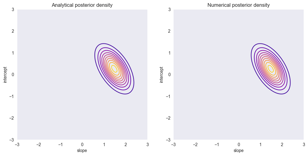
Combining all of the above
All the functions implemented above are used to compute the posterior distribution for various sizes of . The cell below analyses the data set using data points, where the columns visualise (i) data and sample functions, (ii) the prior, (iii) the likelihood and (iv) posterior.
def generate_mvn_samples(mu, Sigma, M):
    """ return samples from a multivariate normal distribution N(mu, Sigma)

    Arguments:
    mu      -- (Dx1) mean vector
    Sigma   -- (DxD) covariance matrix
    M       -- (scalar) number of samples

    Returns:
    (DxM) matrix, where each column corresponds to a sample
    """

    jitter = 1e-8
    D = len(mu)
    L = np.linalg.cholesky(Sigma + jitter*np.identity(D))
    zs = np.random.normal(0, 1, size=(D, M))
    fs = mu + np.dot(L, zs)
    return fs

def compute_f_posterior(x, mu, Sigma):
    """ compute the posterior distribution of f(x) wrt. posterior distribution N(mu, Sigma)

    Arguments:
    x      -- (Nx1) vector of inputs
    mu     -- (2x1) mean vector
    Sigma  -- (2x2) covariance matrix

    Returns:
    mu_f   -- (Nx1) vector of pointwise posterior means at x
    var_f  -- (Nx1) vector of pointwise posterior variances at x

    """

    X = np.column_stack((x, np.ones(len(x))))
    mu_f = np.dot(X, mu)
    var_f = np.diag(np.dot(np.dot(X, Sigma), X.T))[:, None]

    return mu_f, var_f

def plot_prior_density(m, S, a, b):generate_mvn_samplessamples from a multivariate normal by computing a Cholesky factorL = np.linalg.cholesky(Sigma + jitter*np.identity(D)), where a smalljitterterm ensures that is numerically positive definite.Standard normal samples
zsare drawn withnp.random.normal(0, 1, size=(D, M)), giving a matrix of i.i.d. variables; multiplying byLlinearly transforms them to have covariance .The final samples are constructed as
fs = mu + np.dot(L, zs), implementing ; this uses NumPy broadcasting to add the (D)-dimensional mean vectormuto each of the (M) sample columns.In
compute_f_posterior, the design matrixX = np.column_stack((x, np.ones(len(x))))encodes a linear model , with the first column for the input and the second column for the intercept term.Given a posterior over weights , the induced posterior over function values is ; this is implemented by
mu_f = np.dot(X, mu)for the mean.The pointwise posterior variances are the diagonal elements of ; these are extracted via
np.diag(np.dot(np.dot(X, Sigma), X.T))[:, None], with[:, None]reshaping the vector into an column.
Source
import gaussian_linear_regression as glr

# New data set with more data points
np.random.seed(21340)
N_2 = 20
x_2 = np.array([1.764, 0.4, 0.979, 2.241, 1.868, -0.977,  0.95, -0.151, -0.103, 0.411, 0.144, 1.454, 0.761, 0.122,
              0.444, 0.334, 1.494, -0.205,  0.313, -0.854])[:, None]
y_2 = np.array([-0.464, 2.024, 3.191, 2.812, 6.512, -3.022, 1.99, 0.009, 2.513, 3.194, 0.935, 3.216, 0.386, -2.118,
               0.674, 1.222, 4.481, 1.893, 0.422, -1.209])[:, None]
xp = np.linspace(-3, 3, 50)[:, None]

a = np.linspace(-3,3,100)
b = np.linspace(-3,3,100)

def plot_BLR(n=2):
    # compute posterior & generate samples
    mu, Sigma = glr.compute_posterior(x_2[:n, :], y_2[:n, :], m, S, sigma2)
    ahat, bhat = glr.generate_mvn_samples(mu, Sigma, M=30)

    # plot
    plt.figure(figsize=(20, 10))

    plt.subplot2grid((1, 4), (0, 0))
    plt.plot(x_2[:n, :], y_2[:n, :], 'k.', markersize=12)
    plt.ylabel('N = %d' % n, fontweight='bold')
    for (ai, bi) in zip(ahat, bhat):
        plt.plot(xp, glr.predict(xp, ai, bi), 'b-', alpha=0.25)
    mu_f, var_f = glr.compute_f_posterior(xp, mu, Sigma)
    std_f = np.sqrt(var_f)
    plt.plot(xp, mu_f, 'r')
    plt.plot(xp, mu_f + 2*std_f, 'r--')
    plt.plot(xp, mu_f - 2*std_f, 'r--')
    plt.ylim((-6, 6))
    plt.title('Data points', fontweight='bold')
    plt.gca().set_box_aspect(1)
    plt.grid()

    plt.subplot2grid((1, 4), (0, 1))
    glr.plot_prior_density(m, S, a, b)
    plt.title('Prior', fontweight='bold')
    plt.gca().set_aspect('equal', adjustable='box')
    plt.grid()

    plt.subplot2grid((1, 4), (0, 2))
    glr.plot_likelihood(x_2[:n, :], y_2[:n, :], sigma2, a, b)
    plt.title('Likelihood', fontweight='bold')
    plt.gca().set_aspect('equal', adjustable='box')
    plt.grid()

    plt.subplot2grid((1, 4), (0, 3))
    glr.plot_posterior_density(x_2[:n, :], y_2[:n, :], m, S, sigma2, a, b)
    plt.plot(ahat, bhat, 'b.', markersize=10)
    plt.title('Posterior', fontweight='bold')
    plt.gca().set_aspect('equal', adjustable='box')
    plt.grid()

    plt.show()

plot_BLR(n=2)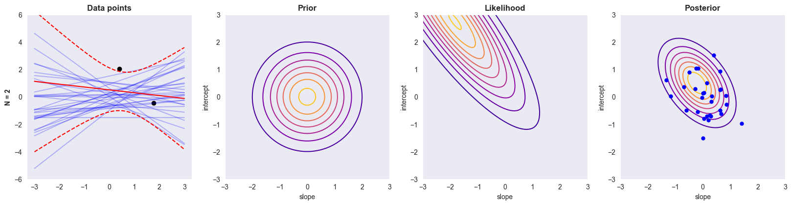
The Quiz
1. How does the blue lines in the first column relate to the blue dots in the fourth column?
Each blue line in the first column is a straight line in the form of linear regression: , whose parameters slope and intercept correspond to one blue point in the fourth column, which is a pair of slope and coefficient in the posterior contour.
2. What happens as the number of samples increase?
Prior contours stay the same as the number of samples increases.
Likelihood contours become dramatically narrower as the number of samples increase
Posterior contours becomes smaller like likelihood contours, but not so significant as the number of samples increases.
Posterior draws: the range of the posterior draws becomes narrower, which tries to fit the data as much as possible as the number of samples increases.
The reason for this behavior is the following: more data points imply more information, which helps reduce uncertainty in regression and makes likelihood and posterior draws narrower
3. Why does the prior have so little effect in the last row?
The amount of data overwhelms the prior: in the last case, the amount of data available is large enough such that the likelihood completely overwhelms the prior, making the prior effect negligible in posterior draws.
Prior is not informative: If the prior is not informative, i.e., it does not provide much useful information about the distribution of the parameters, then it is unlikely to have a significant effect on the posterior. This is true in this case as the prior has zero mean and variance of one, which provideds little prior knowledge about the underlying data structure when there are many datapoints already.
House Price Example
# House Price Dataset

x = np.array([50,55,59,61,79,81,88,90,91,97,99,105,107,110,111,112,116,117,121,123,124,125,135,141, 142,144,145,149, 150,151])
y = np.array([0.36,0.37,0.28,0.29,0.3, 0.5,0.58,0.61,0.62,0.78,0.77,0.83,0.78,0.84,0.91,0.95,1.05,0.99,0.97,0.93,0.81, 0.9,1.1, 0.98, 0.88, 1.05, 1.02, 1.1, 1.08, 1.12])
Source
plt.figure()
plt.scatter(x,y, label='Data points', color='k')
plt.ylabel("Price", fontsize=16)
plt.xlabel("Area [$m^2$]", fontsize=16)
plt.xlim((40, 170))
plt.ylim((0, 1.3))
plt.xticks(fontsize=16)
plt.yticks(fontsize=16)
plt.text(70, 0.35, "?", fontsize=30, color='blue', ha='center')
plt.text(160, 1.05, "?", fontsize=30, color='blue', ha='center')
plt.grid()
plt.legend(loc='lower right', fontsize=16)
plt.tight_layout()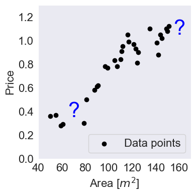
Source
# Noise of prior distribution
m = np.zeros((2, 1))
S = np.eye(2)*[0.1,0.1]
sigma2 = 0.3
print(S)
[[0.1 0. ]
[0. 0.1]]
Source
import gaussian_linear_regression as glr

a_array = np.linspace(-0.001,0.02,200)
b_array = np.linspace(-1,1,200)

A_array, B_array = np.meshgrid(a_array, b_array)
Z = np.array([glr.log_prior(ai, bi, m, S) for (ai, bi) in zip(A_array.ravel(), B_array.ravel())])
Z = Z.reshape((len(a_array), len(b_array)))

plt.figure(figsize=(4,4))
plt.contour(a_array, b_array, glr.log_to_density(Z), cmap='plasma')
plt.xlabel('slope')
plt.ylabel('intercept')
plt.title('Prior')
plt.grid()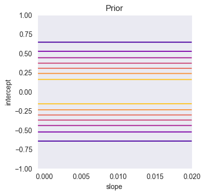
Source
import gaussian_linear_regression as glr

A_array, B_array = np.meshgrid(a_array, b_array)
Z = np.array([glr.log_likelihood(x, y, ai, bi, sigma2) for (ai, bi) in zip(A_array.ravel(), B_array.ravel())])
Z = Z.reshape((len(a_array), len(b_array)))

plt.figure(figsize=(4,4))
plt.contour(a_array, b_array, glr.log_to_density(Z), 10, cmap='plasma')
plt.xlabel('slope')
plt.ylabel('intercept')
plt.title('Likelihood')
plt.grid()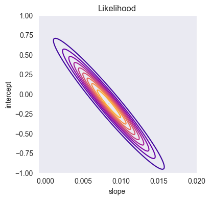
Source
import gaussian_linear_regression as glr

A_array, B_array = np.meshgrid(a_array, b_array)
Z = np.array([glr.log_posterior(x, y, ai, bi, m, S, sigma2) for (ai, bi) in zip(A_array.ravel(), B_array.ravel())])
Z = Z.reshape((len(a_array), len(b_array)))

plt.figure(figsize=(4,4))
plt.contour(a_array, b_array, glr.log_to_density(Z), 10, cmap='plasma')
plt.xlabel('slope')
plt.ylabel('intercept')
plt.title('Posterior')
plt.grid()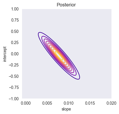
Source
import gaussian_linear_regression as glr

mu, Sigma = glr.compute_posterior(x[:,None], y[:, None], m, S, sigma2)

xp = np.linspace(40, 200, 50)
mu_f, var_f = glr.compute_f_posterior(xp, mu, Sigma)
std_f = np.sqrt(var_f)
mu_f = mu_f.reshape(-1)
std_f = std_f.reshape(-1)

plt.figure(figsize=(12,4))
plt.plot(x, y, 'k.', markersize=12);
plt.plot(xp, mu_f, 'b', label='mean prediction')
plt.fill_between(xp, mu_f - 2*std_f, mu_f + 2*std_f, alpha=0.2, color='r', label='Posterior credibility region')
plt.xlabel('Area [$m^2$]')
plt.ylabel('Price')
plt.legend()
plt.grid()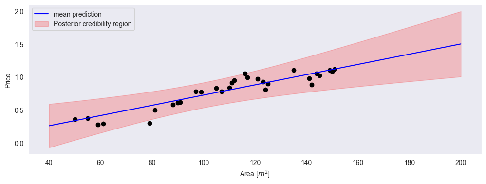
Source
var_y = var_f + sigma2

std_y = np.sqrt(var_y)
mu_f = mu_f.reshape(-1)
std_y = std_y.reshape(-1)

plt.figure(figsize=(12, 4))
plt.plot(x, y, 'k.', markersize=12, label='observations')
plt.plot(xp, mu_f, 'b', label='predictive mean')
plt.fill_between(
    xp,
    mu_f - 2 * std_y,
    mu_f + 2 * std_y,
    alpha=0.2,
    color='r',
    label='Predictive 95% region'
)
plt.xlabel('Area [$m^2$]')
plt.ylabel('Price')
plt.legend()
plt.grid()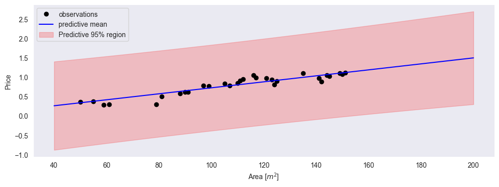
Exercises
Problem 1.1 : Modeling Credit data with Simple Linear Regression
In this exercise, you will perform the basic steps of Bayesian linear regression. To this end, you will work with the Credit dataset that you can load with Pandas from credit_data.csv.
a) Data exploration
Load the dataset and display the first five rows. Identify the predictor () and the response () variables.
Source
credit_df = pd.read_csv('data/credit_data.csv')
credit_df.head(5)= Limit
= Balance
b) Data visualization
Plot the data points of Balance vs. Limit. Describe the relationship you observe. Does a linear model seem appropriate?
Source
plt.scatter(credit_df['Limit'], credit_df['Balance'])
plt.xlabel('Limit')
plt.ylabel('Balance')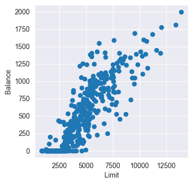
The relationship appears to be linear - except for points close to zero. They seem rather arbitrarily distributed.
c) Model definition
Consider the linear model Explain the meaning of the parameters , , and .
is the slope - change in Balance per unit of Limit
is the intercept - expected Balance when Limit is zero
is the noise variance - the unexplained variation in the data
d) Choosing priors
Plot the prior distribution using the functions derived in the lectures. Assume a Gaussian prior for : , . What does this prior represent? How would the model change if were smaller, such as ? How would that affect the posterior and the predictive region?
Source
a = np.linspace(-2000, 2000, 100)
b = np.linspace(-2000, 2000, 100)

plt.figure(figsize=(10, 4))

m = np.zeros((2, 1))
S = 1e6 * np.identity(2)
plt.subplot(1, 2, 1)
glr.plot_prior_density(m, S, a, b)
plt.title(f"Prior with $\Sigma_p = 10^6 I =$ {S}")

m = np.zeros((2, 1))
S = 1e2 * np.identity(2)
plt.subplot(1, 2, 2)
glr.plot_prior_density(m, S, a, b)
plt.title(f"Prior with $\Sigma_p = 10^2 I =$ {S}")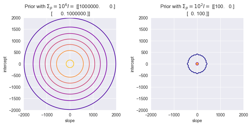
Using smaller diagonal values in means, there is less variance in the parameters. Less variance in turn means that the posterior distribution is more peaked around the true values of and - because there is less uncertainty.
e) Computing the posterior
Plot the likelihood and the posterior distribution using the functions derived in the lectures. Compute the posterior mean and covariance of . Compare and interpret the shapes of the prior, likelihood, and posterior contour plots.
Source
x = credit_df['Limit']
y = credit_df['Balance']

m = np.zeros((2, 1))
S = 1e6 * np.identity(2) # std = 1'000
sigma2 = 1e5 # std of noise ≈ 317

# from scatter plot we expect slope 1250/10'000 ≈ 0.125:
a = np.linspace(0.12, 0.20, 100)
# from scatter plot we expect intercept between 0 and -500,
# from there we fine-tuned the numbers for a nicer plot:
b = np.linspace(-200, -400, 100)

plt.figure(figsize=(10, 4))

plt.subplot(1, 2, 1)
glr.plot_likelihood(x, y, sigma2, a, b)
plt.title(f"Likelihood")
plt.grid()
plt.gca().set_aspect('auto')

plt.subplot(1, 2, 2)
glr.plot_posterior_density(x, y, m, S, sigma2, a, b)
plt.title(f"Posterior")
plt.grid()
plt.gca().set_aspect('auto')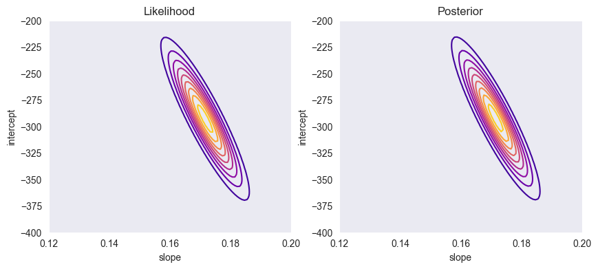
f) Posterior credibility distribution
Using the posterior parameters, calculate the posterior predictive mean and posterior variance: , , and plot these together with the scatter plot. Explain what each component (mean and variance) represents. Explain why the posterior credibility region widens toward the edges of the data.
def plot_posterior_credibility_region(x, y, m, S, sigma2, xp):
    mu, Sigma = compute_posterior(x, y, m, S, sigma2)
    mu_f, var_f = compute_f_posterior(xp, mu, Sigma)

    std_f = np.sqrt(var_f)
    mu_f = mu_f.reshape(-1)
    std_f = std_f.reshape(-1)

    plt.figure(figsize=(12, 4))
    plt.plot(x, y, 'k.', markersize=12, label='observations')
    plt.plot(xp, mu_f, 'b', label='mean prediction')
    plt.fill_between(xp, mu_f - 2 * std_f, mu_f + 2 * std_f, alpha=0.2, color='r', label='Posterior credibility region')
    plt.legend()
    plt.grid()
Source
import gaussian_linear_regression as glr

x = credit_df['Limit']
y = credit_df['Balance']

m = np.zeros((2, 1))
S = 1e6 * np.identity(2) # std = 1'000
sigma2 = 1e5 # std of noise ≈ 317

xp = np.linspace(0, 14_000, 100)
glr.plot_posterior_credibility_region(x, y, m, S, sigma2, xp)
plt.xlabel('Limit')
plt.ylabel('Balance')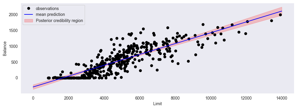
is the most likely linear regression function (the mean of all possible linear functions according to our model)
is the expected uncertainty at every value of x
g) Predictive region
By computing the predictive distribution, plot the predictive region along with the scatter plot. Experiment with different values of (e.g. ). How does changing affect the posterior credibility region and predictive region? Which value seems most reasonable for this dataset?
def plot_predictive_region(x, y, m, S, sigma2, xp):
    mu, Sigma = compute_posterior(x, y, m, S, sigma2)
    mu_f, var_f = compute_f_posterior(xp, mu, Sigma)
    mu_f = mu_f.reshape(-1)

    var_y = var_f + sigma2
    std_y = np.sqrt(var_y)
    std_y = std_y.reshape(-1)

    plt.plot(x, y, 'k.', markersize=12, label='observations')
    plt.plot(xp, mu_f, 'b', label='mean prediction')
    plt.fill_between(
        xp,
        mu_f - 2 * std_y,
        mu_f + 2 * std_y,
        alpha=0.2,
        color='r',
        label='Predictive 95% region'
    )
    plt.legend()
    plt.grid()
Source
import gaussian_linear_regression as glr

x = credit_df['Limit']
y = credit_df['Balance']

m = np.zeros((2, 1))
S = 1e6 * np.identity(2) # std = 1'000
sigmas2 = [1e3, 1e4, 1e5, 1e6] # variance of noise

plt.figure(figsize=(12,22))

xp = np.linspace(0, 14_000, 100)

for i, sigma2 in enumerate(sigmas2):
    plt.subplot(len(sigmas2), 1, i+1)

    glr.plot_predictive_region(x, y, m, S, sigma2, xp)

    plt.xlabel('Limit')
    plt.ylabel('Balance')
    plt.title(f"Noise $\sigma^2 = {sigma2:.0e}$")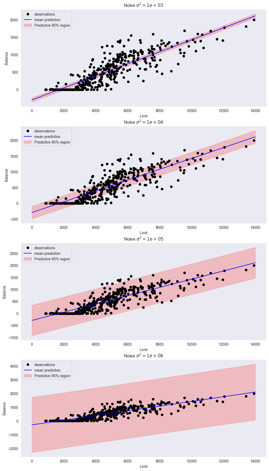
Using looks best; it explains most of the variance and its neither too broad nor too narrow.
h) Model performance
Compute and interpret the following metrics for your model: RMSE, MAE, and . What do these values indicate about model accuracy?
def rmse(mu_f, y):
    return np.sqrt(np.mean((y - mu_f)**2))

def mae(mu_f, y):
    return np.mean(np.abs(y - mu_f))

def r2(mu_f, y):
    return 1 - np.mean((y - mu_f)**2) / np.var(y)
import gaussian_linear_regression as glr
x = credit_df['Limit']
y = credit_df['Balance']
m = np.zeros((2, 1))
S = 1e6 * np.identity(2) # std = 1'000
sigmas2 = 1e5 # std of noise ≈ 317
mu, Sigma = glr.compute_posterior(x, y, m, S, sigma2)
mu_f, var_f = glr.compute_f_posterior(x, mu, Sigma)
mu_f = mu_f.reshape(-1)
print(f"Residual Mean Squared Error (RMSE): {glr.rmse(mu_f, y):.2f}")
print(f"Mean Absolute Error (MAE): {glr.mae(mu_f, y):.2f}")
print(f"R^2: {glr.r2(mu_f, y):.2f}")Residual Mean Squared Error (RMSE): 233.01
Mean Absolute Error (MAE): 177.27
R^2: 0.74
i) Model comparison
Suppose we add a polynomial term to the model. How might this affect the results? Would Bayesian regression still prevent overfitting?
A polynomial model is more powerfull, but risks overfitting. Choosing a corresponding Bayesian prior can act as a regularization technique to prevent overfitting.
j) Reflection
Summarize how the prior, likelihood, and posterior interact. How do and influence the model predictions and uncertainty? Why is it important to interpret both the point estimates and the uncertainty bands when communicating regression results?
The prior describes the belief before seeing any data (our parameter initializations), the likelihood describes the probability of observing the given data using our belief (aka. parameters) and finally the posterior is our updated belief (parameters) after we’ve seen the data.
The describes the uncertainty of our prior (belief): Its diagonal values describe the variance for each parameter (higher variance = higher std. = higher uncertainty).
Lastly, describes the noise in our data (aka. aspects our model cannot explain). This covers the overall predictive uncertainty.
Bayesian linear regression with Bambi
Bambi is a high-level interface for Bayesian regression models built on top of PyMC. It uses an R-style formula interface.
For simple linear regression of body fat on BMI, one might specify
import bambi as bmb

model = bmb.Model("BodyFat ~ BMI", data=df)
results = model.fit()
Conceptually, this is equivalent to specifying the normal linear model
with weakly informative priors chosen automatically for , , and .
Bambi:
Builds the corresponding PyMC model and runs MCMC,
Returns posterior samples in an
InferenceDataobject,Provides tools for posterior summaries, HDIs, and predictive intervals.
More complex models (multiple predictors, categorical variables, interactions, non-normal likelihoods) can be specified by extending the formula or choosing a different family (likelihood).
Posterior HDIs for regression coefficients
From the posterior samples of regression coefficients, we can compute highest density intervals (HDIs).
For a coefficient and a desired probability mass (e.g. 0.90 or 0.94), the -HDI is an interval such that
,
posterior density inside the interval is higher than outside.
Practical interpretation:
If a HDI for does not include zero, we say that zero is not a plausible value for under the model and prior. In informal language: the effect is “significant at the 94% level”.
If the HDI does include zero, then values on both sides (positive and negative effect) are compatible with data and prior; we cannot confidently say the effect is non-zero.
Bambi and ArviZ compute HDIs directly from the posterior samples.
Bayesian for regression
In classical linear regression, the coefficient of determination measures the fraction of variance explained by the model.
In a Bayesian setting, we can define a Bayesian (Gelman et al.), based on posterior samples.
For each posterior draw :
Compute the vector of predicted means (fitted values)
Compute residuals
Compute the explained variance and residual variance for draw :
where the variance is over data points .
Define the per-draw as
The Bayesian is then summarized by the posterior distribution of , e.g. by its mean and an HDI.
This approach acknowledges:
Uncertainty in the regression function (epistemic),
Uncertainty in the noise (aleatoric).
Multiple linear regression
With predictors, the linear regression model generalizes to
In matrix notation:
where now is an matrix (including the intercept column of ones).
Bayesian multiple linear regression:
Place a prior on the coefficient vector and ,
Use MCMC (via PyMC/Bambi) to obtain posterior samples ,
Summarize and interpret parameter and predictive uncertainty.
Adding predictors generally:
Increases the potential explained variance,
Increases epistemic uncertainty (more parameters to estimate),
Risks overfitting if not regularized or if model is too flexible for the data size.
Categorical predictors and interactions
Categorical predictors (e.g. Student yes/no, or Ethnicity with several categories) are incorporated via dummy variables.
Example: binary predictor Student (0 = no, 1 = yes):
shifts the mean response up or down for students compared to non-students.
Interactions between predictors allow the effect of one predictor to depend on another.
For two continuous predictors (TV budget) and (radio budget), a model with interaction is
captures synergy (if positive) or redundancy (if negative) between channels.
In Bambi’s formula syntax:
Main effects:
Sales ~ TV + radioWith interaction:
Sales ~ TV * radio
where TV * radio expands to TV + radio + TV:radio.
Robust linear regression with Student’s likelihood
The normal likelihood is sensitive to outliers: large residuals are heavily penalized, which can pull the regression line towards outlying points.
To reduce sensitivity to outliers, we can model residuals with a Student’s distribution:
where
is the degrees of freedom parameter (shape),
smaller yields heavier tails than the normal distribution.
As , the Student’s distribution converges to the normal:
A Bayesian robust regression model might use:
Normal priors for coefficients ,
A prior on (half-normal, exponential, etc.),
A prior on (e.g. ).
Compared to the normal-likelihood model, the -likelihood:
Gives less weight to extreme residuals,
Produces regression lines less distorted by outliers,
Often yields broader predictive intervals, reflecting uncertainty about outliers.
Polynomial regression
To capture simple nonlinear relationships between a single predictor and response , we can use polynomial regression.
For a degree-3 polynomial:
This is still linear in the parameters , so it fits into the linear regression framework by defining transformed predictors:
However:
Polynomial terms can be strongly correlated (e.g. and ), causing numerical issues.
High-degree polynomials can overfit heavily, especially with few data points.
Bambi’s poly(x, d) construct can create orthogonal polynomials, which reduce the correlations between polynomial
terms and improve sampling stability.
Overfitting and epistemic uncertainty in polynomial models
With few data points and a highly flexible model (e.g. high-degree polynomial), the model can fit the training data very closely, but:
The regression function becomes wiggly and unstable,
Posterior predictive intervals can become very wide away from data points,
Epistemic uncertainty increases, reflecting that many different polynomials are compatible with the data.
Bayesian inference:
Makes overfitting visible in the posterior distribution of functions and predictive intervals,
Encourages the use of priors (shrinkage) to regularize complex models,
Allows the use of model comparison (e.g. Bayes factors, ELPD) to decide whether increased flexibility is justified.
Shrinkage via normal priors and L2 regularisation
Consider a linear regression model with predictors (possibly including polynomial terms) and coefficients . Suppose we place an independent normal prior on each coefficient:
and a normal likelihood
Ignoring constants, the log posterior is
Up to additive constants, this becomes
The maximum a posteriori (MAP) estimate maximizes this log posterior, i.e. minimizes
Up to a constant factor, this is equivalent to ridge regression (L2 regularisation):
with penalty parameter .
Thus:
L2 regularisation corresponds to a normal prior on coefficients centered at zero.
Stronger prior shrinkage (smaller ) corresponds to larger and stronger penalization of large coefficients.
L1 regularisation and Laplace prior
Analogously, L1 regularisation (lasso) corresponds to a Laplace (double-exponential) prior on the coefficients.
The Laplace prior for a scalar coefficient with scale has density
Ignoring constants, the log prior is
so for a vector of coefficients with independent Laplace priors, the negative log prior adds a term proportional to .
The MAP estimator then minimizes
which is the lasso objective.
In summary:
Normal prior on ridge (L2) penalty at MAP.
Laplace prior on lasso (L1) penalty at MAP.
Regularisation can therefore be understood as a natural consequence of using informative priors in Bayesian models.
Model selection versus regularisation
When dealing with flexible models (e.g. polynomials of various degrees), there are two complementary strategies:
Model selection
Compare several models (e.g. linear, quadratic, cubic) using:Bayes factors (marginal likelihoods),
ELPD / LOO,
Posterior predictive checks,
Predictive RMSE/MAE.
Then choose the model that best balances fit and complexity.
Regularisation (shrinkage)
Use a richer model (e.g. higher-degree polynomial) but place strong priors that shrink higher-order coefficients towards zero. This keeps the model flexible but penalizes unnecessary complexity.
Often, a combination of both is used:
Start with a simple model,
Add complexity if strongly supported by posterior predictive checks and model comparison,
Use priors to regularize complex models and avoid overfitting.
In Bayesian regression, regularisation is not an ad-hoc fix but an integral part of the modelling philosophy through the choice of priors.