Simple Linear Regression

Simple Linear Regression Model ^[1]¶

Simple linear regression lives up to its name: it is a very straightforward approach for predicting a quantitative response $Y$ on the basis of a single predictor variable $X$ . It assumes that there is approximately a linear relationship between $X$ and $Y$ . Mathematically, we can write this linear relationship as

You might read “ $\approx$ ” as “is approximately modeled as”. We will sometimes describe this equation by saying that we are regressing $Y$ on $X$ (or $Y$ onto $X$ ).

Using statsmodels ^[2]¶

We are interested in the values of $\hat{\beta}_{0}$ and $\hat{\beta}_{1}$ for the Advertising data. By means of the Python-function OLS(), we can easily determine those values:

import pandas as pd
import statsmodels.api as sm

# Load data
df = pd.read_csv('data/Advertising.csv')
x = df['TV']
y = df['sales']

# Linear Regression using statsmodels.api
x_sm = sm.add_constant(x)
model = sm.OLS(y, x_sm).fit()

# Now we can print a summary, 
print(model.summary())

                            OLS Regression Results                            
==============================================================================
Dep. Variable:                  sales   R-squared:                       0.612
Model:                            OLS   Adj. R-squared:                  0.610
Method:                 Least Squares   F-statistic:                     312.1
Date:                Wed, 02 Mar 2022   Prob (F-statistic):           1.47e-42
Time:                        08:34:12   Log-Likelihood:                -519.05
No. Observations:                 200   AIC:                             1042.
Df Residuals:                     198   BIC:                             1049.
Df Model:                           1                                         
Covariance Type:            nonrobust                                         
==============================================================================
                 coef    std err          t      P>|t|      [0.025      0.975]
------------------------------------------------------------------------------
const          7.0326      0.458     15.360      0.000       6.130       7.935
TV             0.0475      0.003     17.668      0.000       0.042       0.053
==============================================================================
Omnibus:                        0.531   Durbin-Watson:                   1.935
Prob(Omnibus):                  0.767   Jarque-Bera (JB):                0.669
Skew:                          -0.089   Prob(JB):                        0.716
Kurtosis:                       2.779   Cond. No.                         338.
==============================================================================

Notes:
[1] Standard Errors assume that the covariance matrix of the errors is correctly specified.

The coefficients are listed under (coef). Here const corresponds to $\hat{\beta}_{0}$ , thus to the intercept with the $y$ -axis, and the TV corresponds to the slope of the regression line, thus to $\hat{\beta}_{1}$ .

Using sklearn¶

import numpy as np
from sklearn.linear_model import LinearRegression

x = [[x[i]] for i in range(len(x))]

# Linear Regression using sklearn
linreg = LinearRegression()
linreg.fit(x, y)

print('Coefficients: \n', np.round(linreg.coef_, 4),
      '\nIntercept: \n', np.round(linreg.intercept_, 4))

Coefficients: 
 [0.0475] 
Intercept: 
 7.0326

Our regression model then is given by

Y \approx 7.03+0.0475X

According to this approximation, an additional CHF 1000 spent on TV advertising is associated with selling approximately 47.5 additional units of the product.

import matplotlib.pyplot as plt

# Predicted y
y_pred = model.predict(x_sm)

# Create figure and plot
fig = plt.figure(figsize=(6, 6))
ax = fig.add_subplot(1, 1, 1)
plt.plot(df['TV'], y, marker='o', linestyle='None', 
         color='darkcyan', markersize='3', label="Data")
plt.plot(df['TV'], y_pred, 'b-', label="Predction")
# Set labels and Legend
ax.set_xlabel('TV')
ax.set_ylabel('Sales')
plt.legend()
plt.show()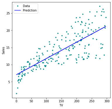

The Python-function statsmodels.api.OLS() uses Ordinary Least Squares to fit the linear model.
Be aware of the (default) order of the function parameters x and y in sm.OLS(y, x).
If x is a one-dimensional vector, it needs to be preprocessed using sm.add_constant(x).

np.sqrt(model.mse_resid)

3.258656368650463

Hypothesis Tests and Confidence Intervals¶

Assessing the Accuracy of the Coefficient Estimates ^[3]¶

Recall that we assume that the true relationship between $X$ and $Y$ takes the form

Y = f(X) + \varepsilon

(2)

for some unknown function $f$ , where $\varepsilon$ is a mean-zero random error term. If $f$ is to be approximated by a linear function, then we can write this relationship as

Y = \beta_0 + \beta_1 X + \varepsilon

(3)

Here $\beta_0$ is the intercept term — that is, the expected value of $Y$ when $X = 0$ , and $\beta_1$ is the slope — the average increase in $Y$ associated with a one-unit increase in $X$ . The error term is a catch-all for what we miss with this simple model:

the true relationship is probably not linear,
there may be other variables that cause variation in $Y$ ,
there may be measurement error.

The central limit theorem tells us that the sum of all those random variables is approximately distributed according to a normal distribution. Furthermore, we typically assume that the error term is independent of $X$ .

Example ^[4]¶

In this example we assume that we know the true relationship between $X$ and $Y$ , which is

f(X) =2+3X

(4)

However, in practice we will never observe this perfect relationship, but

Y=f(X)+\epsilon =2+3X +\epsilon

(5)

We call $f(X)=2+3x$ the population regression line, which is the best linear approximation to the true relationship between $X$ and $Y$ . If we now observe realizations of $X$ and $Y$ , we can determine the least squares line

Y=\beta_0 + \beta_1 X + \epsilon

by estimating $\beta_0$ and $\beta_1$ according to the equation.

Let us simulate the observed data $X$ and $Y$ from the model

Y=2+3X+\epsilon

where $\epsilon$ is normally distributed with mean 0, thus $\epsilon\sim\mathcal{N}(0,\sigma^{2})$ . We create 100 random values of $X$ , and generate 100 corresponding values of $Y$ from the model $Y=2+3X+\epsilon$

import numpy as np

n = 100  # number of datapoints

# crate data around y=ax+b
a, b = 3, 2
x = np.sort(np.random.uniform(low=-2, high=2, size=(n)))

y = b + a*x + np.random.normal(loc=0.0, scale=4, size=n)


x_true = np.linspace(-2, 2, n)
y_true = b + a*x_true

We can now plot a number of randomly generated datapoints and the found regression line.

import matplotlib.pyplot as plt
import statsmodels.api as sm

# Create figure and plot
fig = plt.figure(figsize=(14, 4))
for i in range(3):
    ax = fig.add_subplot(1, 3, i+1)
    
    # Random data along known function:
    x = np.sort(np.random.uniform(low=-2, high=2, size=n))
    x_sm = sm.add_constant(x)
    y = 2 + 3*x + np.random.normal(loc=0.0, scale=4, size=n)
    # Linear Regression and prediction:
    model = sm.OLS(y, x_sm).fit()
    y_pred = model.predict(x_sm)
    
    # Data points:
    plt.plot(x, y, marker='o', linestyle='None', 
             color='darkcyan', markersize='3', label="Data")
    # True line:
    plt.plot(x_true, y_true, 'r-', label="True")
    # Predicted line:
    plt.plot(x, y_pred, 'b-', label="Prediction")

    # Set labels and Legend
    ax.set_xlabel('x'), ax.set_ylabel('y')
    ax.set_xlim(-2, 2), ax.set_ylim(-10, 10)
    plt.legend()

plt.tight_layout()
plt.show()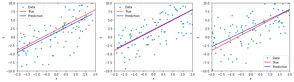

The red line represents the plot of the function $f(X)=2+3X$ , which remains identical in all three simulations. The blue line is the least squares line that was constructed by means of the least squares estimates for the simulated data. Each least squares line is different, but on average, the least squares lines are quite close to the population regression line.

In the next figure we have generated ten different data sets from the model given by $Y = 2+3X +\epsilon$ and plotted the corresponding ten least squares lines. Notice that different data sets generated from the same true model result in slightly different least squares lines, but the unobserved population regression line does not change.

n_lines = 100 # number of iterations

# Create figure and plot
fig = plt.figure(figsize=(6,4))
ax = fig.add_subplot(1, 1, 1)

for i in range(n_lines):
    # Random data allong known function:
    x = np.sort(np.random.uniform(low=-2, high=2, size=n))
    x_sm = sm.add_constant(x)
    y = 2 + 3*x + np.random.normal(loc=0.0, scale=4, size=n)
    # Linear Regression and prediction:
    model = sm.OLS(y, x_sm).fit()
    y_pred = model.predict(x_sm)

    # Predicted line:
    plt.plot(x, y_pred, 'b-', alpha=0.7)
# True line:
plt.plot(x_true, y_true, 'r-', label="True")
# Set labels and Legend
ax.set_xlabel('x'), ax.set_ylabel('y')
ax.set_xlim(-2, 2), ax.set_ylim(-10, 10)

plt.show()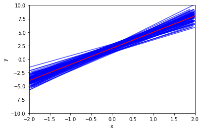

Example ^[5]¶

For the Advertising data we can determine the standard errors of the estimated coefficients with the help of Python:

import pandas as pd
import statsmodels.api as sm

# Load data
df = pd.read_csv('data/Advertising.csv')
x = df['TV']
y = df['sales']

# Linear Regression using statsmodels.api
x_sm = sm.add_constant(x)
model = sm.OLS(y, x_sm).fit()

# Now we can print a summary, 
print(model.summary())

                            OLS Regression Results                            
==============================================================================
Dep. Variable:                  sales   R-squared:                       0.612
Model:                            OLS   Adj. R-squared:                  0.610
Method:                 Least Squares   F-statistic:                     312.1
Date:                Fri, 25 Feb 2022   Prob (F-statistic):           1.47e-42
Time:                        17:56:43   Log-Likelihood:                -519.05
No. Observations:                 200   AIC:                             1042.
Df Residuals:                     198   BIC:                             1049.
Df Model:                           1                                         
Covariance Type:            nonrobust                                         
==============================================================================
                 coef    std err          t      P>|t|      [0.025      0.975]
------------------------------------------------------------------------------
const          7.0326      0.458     15.360      0.000       6.130       7.935
TV             0.0475      0.003     17.668      0.000       0.042       0.053
==============================================================================
Omnibus:                        0.531   Durbin-Watson:                   1.935
Prob(Omnibus):                  0.767   Jarque-Bera (JB):                0.669
Skew:                          -0.089   Prob(JB):                        0.716
Kurtosis:                       2.779   Cond. No.                         338.
==============================================================================

Notes:
[1] Standard Errors assume that the covariance matrix of the errors is correctly specified.

In the table under coef, the listed values are $\hat{\beta}_{0}$ and $\hat{\beta}_{1}$ . In the column Std.,Error we find the values $0.457843$ and $0.002691$ for the two standard errors $se (\hat{\beta}_{0})$ and $se (\hat{\beta}_{1})$ . They correspond to the average deviations of the estimated values of $\hat{\beta}_{0}$ and $\hat{\beta}_{1}$ which are $7.0326$ and $0.04754$ . In the right top part, we find some constants describing the fit, for example R-squared which is the portion of variance explained by the fit.

Hypothesis Test¶

Example ^[6]¶

For the Advertising data, we want to compute the p-value of $\beta_1$ of the least squares model for the regression of number of units sold on TV advertising budget.

The least squares estimate for $\beta_1$ is 0.047537 and the standard error of $\hat{\beta}_1$ .

Hence, we find for the realization of the statistic $T$

t =\dfrac{\hat{\beta}_{1}-0}{se (\hat{\beta}_{1})} =\dfrac{0.047537-0}{0.002691} =17.66518

Furthermore, we find in the Python-output, that the number of degrees of freedom is 198, which is listed under Df Residuals. The number of degrees of freedom is given by $n-2$ , it follows that in total there are $n=200$ data points. This number corresponds to the number of markets in the data set Advertising.

Since the coefficient for $\hat{\beta}_1$ is very large relative to its standard error, so the t-statistic is also large. The probability of seeing such a value if $H_{0}$ is true is virtually zero. Hence we can conclude that $\beta_{1}\neq 0$ .

We now will compute the p-value, that is, the probability of observing a value of the t-statistic larger than $|t|=17.66518$ . Assuming $\beta_1=0$ , $T$ will follow a t-distribution with $n-2=198$ degrees of freedom. Then the (two-sided) p-value can be determined with the help of *Python

from scipy.stats import t

p_two_sided = 2 * (1 - t.cdf(17.66518, 198))
print(p_two_sided)

0.0

Since the alternative hypothesis is two-sided, we need to multiply the one-sided p-value by two in order to obtain the two-sided p-value. The corresponding p-value : 0.000 is listed under P(>|t|). Since it is zero, hence smaller than a siginificance level of $0.05$ , we reject the null hypothesis $\beta_{1}=0$ in favor of the alternative hypothesis $\beta_{1}\neq 0$ . We therefore find that there clearly is a relationship between TV and sales.

Confidence Intervals for Regression Coefficients¶

Example ^[7]¶

In the case of the Advertising data, the 95% confidence interval can be found with the help of the conf_int-function:

import numpy as np
# Confidence interval found using conf_int method
print(np.round(model.conf_int(alpha=0.05), 4))

            0       1
const  6.1297  7.9355
TV     0.0422  0.0528

The 95%-confidence interval for $\beta_{0}$ thus is

[6.130,7.935]

and the 95%-confidence interval for $\beta_{1}$

[0.042,0.053]

Therefore, we can conclude that in the absence of any advertising, sales will, on average, fall somewhere between $6130$ and $7935$ units. Furthermore, for each CHF 1000 increase in television advertising, there will be an average increase in sales of between 42 and 53 units.

The exact formula for the 95% confidence interval for the regression coefficient $\beta_i$ is

\left [ \hat{\beta}_i- t_{0.975;n-2}\cdot se (\hat{\beta}_{i}),\hat{\beta}_{i}+ t_{0.975;n-2}\cdot se (\hat{\beta}_{i}) \right ]

where $t_{0.975;n-1}$ is the 97.5% quantile of a t-distribution with $n-2$ degrees of freedom.

With Python we determine the 97.5% quantile of a t-distribution as follows

# the 97.5% quantile of a t-distribution:
q_975 = t.ppf(0.975, 18)
print(np.round(q_975, 4))

2.1009

which is approximately 2.

Confidence and Prediction Intervals for the Response¶

Example ^[8]¶

For the Advertising data set we determine the 95% confidence intervals for the following values of TV : $3$ , $100$ and $275$

import numpy as np
import pandas as pd
import statsmodels.api as sm

# Load data
df = pd.read_csv('data/Advertising.csv')
x = df['TV']
y = df['sales']

# Fit Linear Model
x = sm.add_constant(x)
model = sm.OLS(y,x).fit()

# Prediction at points 3, 100 and 270
x0 = [3, 100, 275]
x0 = sm.add_constant(x0)

predictionsx0 = model.get_prediction(x0)
predictionsx0 = predictionsx0.summary_frame(alpha=0.05)
predictionsx0 = np.round(predictionsx0, 4)
print(predictionsx0)

      mean  mean_se  mean_ci_lower  mean_ci_upper  obs_ci_lower  obs_ci_upper
0   7.1752   0.4509         6.2860         8.0644        0.6879       13.6626
1  11.7863   0.2629        11.2678        12.3047        5.3393       18.2333
2  20.1052   0.4143        19.2882        20.9221       13.6273       26.5830

In the Python-output, the values

\hat{y}_{0} =\hat{\beta}_{0}+\hat{\beta}_{1}x_{0}

can be found under mean; they correspond to the $y$ -values on the regression line, thus to the predicted response given a predictor value. Under mean ci lower the lower limits, under mean ci upper the upper limits of the corresponding confidence intervals can be found.

For the value $x_{0}=100$ the 95% confidence interval is given by

[11.268,12.305]

The expected value of $\hat{y}_0$ given the predictor value $x_{0}=100$ is contained in this interval with a probability of 95%.

We can visualize confidence intervals for the expected response variable given an intervall of predictor values. In the next figure the regression line is plotted in blue. The green curves correspond to the lower and upper limits of the confidence intervals given a $x_{0}$ . The red lines represent the 95% confidence intervals for the values $x_{0}=3, 100$ and $275$ . These intervals contain with a probability of 95% the corresponding expected values of $\hat{y}_{0}$ .

import matplotlib.pyplot as plt

x = np.linspace(0, 300)
x_sm = sm.add_constant(x)

# Predictions
predictionsx = model.get_prediction(x_sm)
# at 95% confidence:
predictionsx = predictionsx.summary_frame(alpha=0.05)

# Create figure and plot
fig = plt.figure(figsize=(8, 6))
ax = fig.add_subplot(1, 1, 1)
# prediction
plt.plot(x, predictionsx.loc[:,'mean'], 'b-')
# upper and lower boundaries at 95%
plt.plot(x, predictionsx.loc[:,'mean_ci_lower'], 'c-')
plt.plot(x, predictionsx.loc[:,'mean_ci_upper'], 'c-')
# lines of the three points in x0:
for i in range(len(x0)):
    plt.plot([x0[i, 1], x0[i, 1]], 
             [0, predictionsx0.loc[:,'mean_ci_lower'][i]], 'k:' )
    plt.plot([x0[i, 1], x0[i, 1]], 
             [predictionsx0.loc[:,'mean_ci_lower'][i], 
              predictionsx0.loc[:,'mean_ci_upper'][i]], 'r-' )

# Set labels and Legend
ax.set_xlabel('TV')
ax.set_ylabel('Sales')

plt.show()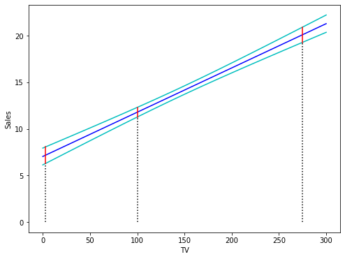

Prediction Intervals¶

Example ^[9]¶

In the case of the Advertising data we determine the 95% prediction intervals for the $x$ -values $3$ , $100$ and $225$ from the same results as provided in the previous example.

Under mean the predicted $y$ -values on the regression line

\hat{y}_{0} =\hat{\beta}_{0}+\hat{\beta}_{1}x_{0}

can be found.

obs ci lower displays the lower limits and obs ci upper the upper limits of the prediction intervals for the given $x$ -values.

For the predictor value $x_{0}=100$ the 95% prediction interval is given by

[5.339,18.233]

A future observation $y_0$ for given $x_{0}=100$ will fall with a probability of 95% into this interval. As we can observe, the prediction interval thus is clearly larger than the confidence interval for the expected value of $\hat{y}_0=\hat{\beta}_0+\hat{\beta}_1 x_{0}$ .

It is again very instructive to visualize the point-wise prediction intervals. The following figure displays the regression line in blue. The green curves represent the upper and lower limits of the prediction intervals for future observations. The red lines correspond to 95% prediction intervals for $x_{0}=3, 100 ,275$ . These intervals contain with a probability of 95% the true values of the corresponding future observations $y_{0}$ .

x = np.linspace(0, 300)
x_sm = sm.add_constant(x)

# Predictions
predictionsx = model.get_prediction(x_sm)
# at 95% confidence:
predictionsx = predictionsx.summary_frame(alpha=0.05)

# Create figure and plot
fig = plt.figure(figsize=(8, 6))
ax = fig.add_subplot(1, 1, 1)
# prediction
plt.plot(x, predictionsx.loc[:,'mean'], 'b-')
# upper and lower boundaries at 95%
plt.plot(x, predictionsx.loc[:,'obs_ci_lower'], 'c-')
plt.plot(x, predictionsx.loc[:,'obs_ci_upper'], 'c-')
# lines of the three points in x0:
for i in range(len(x0)):
    plt.plot([x0[i, 1], x0[i, 1]], 
             [0, predictionsx0.loc[:,'obs_ci_lower'][i]], 'k:' )
    plt.plot([x0[i, 1], x0[i, 1]], 
             [predictionsx0.loc[:,'obs_ci_lower'][i], 
              predictionsx0.loc[:,'obs_ci_upper'][i]], 'r-' )

# Set labels and Legend
ax.set_xlabel('TV')
ax.set_ylabel('Sales')

plt.show()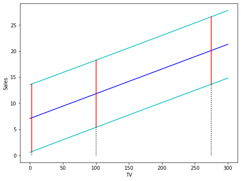

Footnotes¶

Birbaumer et al., 2025, p. 104
↩
Birbaumer et al., 2025, Example 5.2.4
↩
Birbaumer et al., 2025, p. 111
↩
Birbaumer et al., 2025, Example 5.3.1
↩
Birbaumer et al., 2025, Example 5.3.3
↩
Birbaumer et al., 2025, Example 5.3.3
↩
Birbaumer et al., 2025, Example 5.3.3
↩
Birbaumer et al., 2025, Example 5.4.2
↩
Birbaumer et al., 2025, Example 5.4.2
↩

References¶

Birbaumer, M., Frick, K., Büchel, P., & van Hemert, S. (2025). Predictive Modeling - Lecture Notes.

Simple Linear Regression