Logistic Regression
Logistic Regression Example 1.1
The approach results in a model for as depicted(blue line). The probability
is plotted against the monthly credit card bill (balance) . The probabilities of the observed values are given by the -Coding of the default variable: if default=Yes we have (green dots) and in case default=No we have (red dots).
import numpy as np
import pandas as pd
import matplotlib.pyplot as plt
import statsmodels.api as sm

# Load data
df = pd.read_csv('Logistic Regression/data/Default.csv', sep=';')

# Add a numerical column for default
df = df.join(pd.get_dummies(df['default'],
                            prefix='default',
                            drop_first=True))

# Index of Yes:
i_yes = df.loc[df['default_Yes'] == 1, :].index

# Random set of No:
i_no = df.loc[df['default_Yes'] == 0, :].index
i_no = np.random.choice(i_no, replace=False, size=333)

# Fit Linear Model, only including the selection of no
i_ = np.concatenate((i_no, i_yes))
x = df.iloc[i_]['balance']
y = df.iloc[i_]['default_Yes']

x_sm = sm.add_constant(x)
model = sm.OLS(y, x_sm).fit()

# Find the predicted values
x_pred = x.sort_values()
y_pred = model.predict(sm.add_constant(x_pred))
""" Plot """
# Create Figure and subplots
fig = plt.figure(figsize=(7, 4))
ax = fig.add_subplot(111)
# Plot datapoints
plt.plot(df.iloc[i_yes]['balance'], df.iloc[i_yes]['default_Yes'],
'or', alpha=0.5, label='Default=Yes')
plt.plot(df.iloc[i_no]['balance'], df.iloc[i_no]['default_Yes'],
'og', alpha=0.5, label='Default=No')
# Plot fit
plt.plot(x_pred, y_pred, 'b-', label='Linear Regression')
# Labels and limits
ax.set_xlabel('Balance')
ax.set_ylabel('Probability for Default')
ax.set_ylim(-0.1, 1.1)
plt.legend()
plt.show() 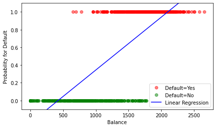
# Define t and p
t = np.arange(-7, 7, 0.1)
p = []
for i in range(len(t)):
    p.append(np.exp(t[i]) / (1 + np.exp(t[i])))

# Plot graph
# Create Figure and subplots
fig = plt.figure(figsize=(7, 4))
ax = fig.add_subplot(111)
plt.plot(t, p, 'r-')
plt.grid(True)
plt.xlabel('t')
plt.ylabel('p')
plt.show()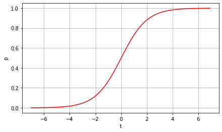
Note that the linear function of the model returns negative values for low balance and values greater than 1 for high balance. These values are not interpretable as probabilities, since those are bounded between 0 and 1.
Also note that only a part of the data was included. The full data contains many more default = No entries, which would result in a much lower probability for default.
Logistic Regression Example 1.2
A simple logistic regression model for the Default data is plotted.
import numpy as np
import pandas as pd
import matplotlib.pyplot as plt
import statsmodels.api as sm

# Load data
df = pd.read_csv('Logistic Regression/data/Default.csv', sep=';')

# Add a numerical column for default
df = df.join(pd.get_dummies(df['default'],
                            prefix='default',
                            drop_first=True))

# Index of Yes:
i_yes = df.loc[df['default_Yes'] == 1, :].index

# Random set of No:
i_no = df.loc[df['default_Yes'] == 0, :].index
i_no = np.random.choice(i_no, replace=False, size=333)

# Fit Linear Model, only including the selection of no
i_ = np.concatenate((i_no, i_yes))
x = df.iloc[i_]['balance']
y = df.iloc[i_]['default_Yes']

x_sm = sm.add_constant(x)

model = sm.GLM(y, x_sm, family=sm.families.Binomial())
model = model.fit()

# Find the predicted values
x_pred = x.sort_values()
y_pred = model.predict(sm.add_constant(x_pred))
""" Plot """
# Create Figure and subplots
fig = plt.figure(figsize=(7, 4))
ax = fig.add_subplot(111)
# Plot datapoints
plt.plot(df.iloc[i_yes]['balance'], df.iloc[i_yes]['default_Yes'],
'or', alpha=0.5, label='Default=Yes')
plt.plot(df.iloc[i_no]['balance'], df.iloc[i_no]['default_Yes'],
'og', alpha=0.5, label='Default=No')
# Plot fit
plt.plot(x_pred, y_pred, 'b-', label='Logistic Regression')
# Labels and limits
ax.set_xlabel('Balance')
ax.set_ylabel('Probability for Default')
ax.set_ylim(-0.1, 1.1)
plt.legend()
plt.show() 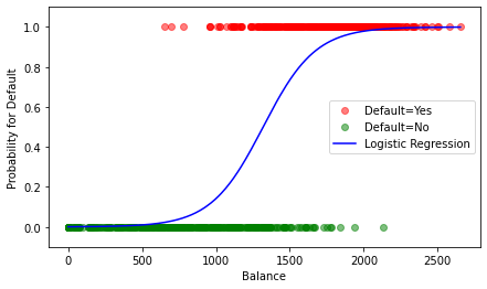
For small values of balance the predicted values for tend to 0. Likewise, the predictions tend to 1 for large balance values. All values of the model are within the interval and thus interpretable as probabilities.
Extra info:
The graph would look rather different if the complete data would be included:
# Fit logistic model, using all no
x = df['balance']
y = df['default_Yes']

x_sm = sm.add_constant(x)

model = sm.GLM(y, x_sm, family=sm.families.Binomial())
model = model.fit()

# Find the predicted values
x_pred = x.sort_values()
y_pred = model.predict(sm.add_constant(x_pred))
""" Plot """
# Create Figure and subplots
fig = plt.figure(figsize=(7, 4))
ax = fig.add_subplot(111)
# Plot datapoints
plt.plot(df.iloc[i_yes]['balance'], df.iloc[i_yes]['default_Yes'],
'or', alpha=0.5, label='Default=Yes')
plt.plot(df.iloc[i_no]['balance'], df.iloc[i_no]['default_Yes'],
'og', alpha=0.5, label='Default=No')
# Plot fit
plt.plot(x_pred, y_pred, 'b-', label='Logistic Regression')
# Labels and limits
ax.set_xlabel('Balance')
ax.set_ylabel('Probability for Default')
ax.set_ylim(-0.1, 1.1)
plt.legend()
plt.show() 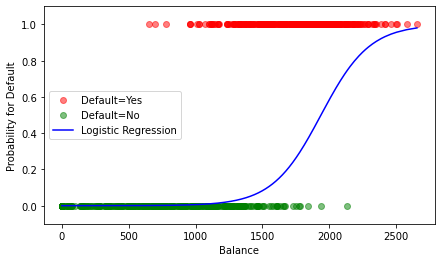
Logistic Regression Example 2.2
The Python-output below shows the estimates for the parameters in the logistic regression model.
import numpy as np
import pandas as pd
import statsmodels.api as sm

# Load data
df = pd.read_csv('Logistic Regression/data/Default.csv', sep=';')

# Add a numerical column for default
df = df.join(pd.get_dummies(df['default'],
                            prefix='default',
                            drop_first=True))

# Fit logistic model
x = df['balance']
y = df['default_Yes']

x_sm = sm.add_constant(x)

model = sm.GLM(y, x_sm, family=sm.families.Binomial())
model = model.fit()

# Print summary
print(model.summary())
Generalized Linear Model Regression Results
==============================================================================
Dep. Variable: default_Yes No. Observations: 10000
Model: GLM Df Residuals: 9998
Model Family: Binomial Df Model: 1
Link Function: logit Scale: 1.0000
Method: IRLS Log-Likelihood: -798.23
Date: Tue, 21 Mar 2023 Deviance: 1596.5
Time: 09:01:21 Pearson chi2: 7.15e+03
No. Iterations: 9
Covariance Type: nonrobust
==============================================================================
coef std err z P>|z| [0.025 0.975]
------------------------------------------------------------------------------
const -10.6513 0.361 -29.491 0.000 -11.359 -9.943
balance 0.0055 0.000 24.952 0.000 0.005 0.006
==============================================================================
# Find confidence interval
print(model.conf_int(alpha=0.05))
0 1
const -11.359208 -9.943453
balance 0.005067 0.005931
The two-sided -interval for is well seperated from 0 which is equivalent to rejecting with a type I error of .
Logistic Regression Example 3.1
The estimated coefficients are
Thus, if an individual has balance = 1000, then the model yields
import numpy as np
import pandas as pd
import statsmodels.api as sm

# Load data
df = pd.read_csv('Logistic Regression/data/Default.csv', sep=';')

# Add a numerical column for default
df = df.join(pd.get_dummies(df['default'],
                            prefix='default',
                            drop_first=True))

# Fit logistic model
x = df['balance']
y = df['default_Yes']

x_sm = sm.add_constant(x)

model = sm.GLM(y, x_sm, family=sm.families.Binomial())
model = model.fit()

# Predict for balance = 1000
x_pred = [1, 1000]
y_pred = model.predict(x_pred)

print(y_pred)
[0.00575215]
This probability of default is well below , which is very low. However, a different individual with balance = 2000 has a default probability of approximately .
# Predict for balance = 2000
x_pred = [1, 2000]
y_pred = model.predict(x_pred)

print(y_pred)
[0.58576937]
Logistic Regression Example 3.2
For the Default data the following Python-code computes the training classification error.
""" Follows Example 3.1 """
# Predict for training data
x_pred = x_sm
y_pred = model.predict(x_pred)
print(y_pred[10])

# Round to 0 or 1
y_pred = y_pred.round()
print(y_pred[10])

# Compute training error
e_train = abs(y - y_pred)
e_train = e_train.mean()

print(e_train)
2.3668765516963852e-05
0.0
0.0275
The value of the training error in this example is 0.0275, which is to say that approximately 97.25% of the cases in the training set are classified correctly.
Logistic Regression Example 3.3
The following Python-code produces the confusion matrix for the Default data set and the logistic regression model.
""" Follows Example 3.2 """
# Create confusion matrix
confusion = pd.DataFrame({'predicted': y_pred,
                          'true': y})
confusion = pd.crosstab(confusion.predicted, confusion.true,
                        margins=True, margins_name="Sum")

print(confusion)
true 0 1 Sum
predicted
0.0 9625 233 9858
1.0 42 100 142
Sum 9667 333 10000
It can be seen that out of 9667 cases with default=No, the vast majority of 9625 are classified correctly. On the other hand, only approximately of the default=Yes cases are classified correctly. The confusion matrix shows that the present classification scheme is by no means useful, in particular, if you want to predict the case of default=Yes.
The reason for this bad result is the imbalance of the two classes. The training data only contains 333 out of cases with default=Yes. Therefore, the likelihood function is dominated by the factors corresponding to default=No, so the parameters are chosen as to match mainly those cases. Note also that the trivial classifier predicting all observations to has a classification error of which is not much worse than that of our logistic model.
The situation can also be visualized by the histograms of the estimated probabilities of default=Yes separated by true class.
It is striking that the default=No group has a high concentration of probabilities near 0 which is reasonable for this group. On the other hand, though, the estimated probabilities for the default=Yes cases do not exhibit high mass at 1. Instead, the maximal probability is attained close to 0 as well!
Logistic Regression Example 3.8
We can compute the F1 score by means of the
""" Follows Example 3.3 """
from sklearn.metrics import f1_score

# Find F1-score
f1 = f1_score(y, y_pred, pos_label=1, average='binary')
print(f1)
0.42105263157894746
pos_label is an optional character string for the factor level that corresponds to a positive result.
Logistic Regression Example 3.9
If we consider the case default=No as positive, then the F1 score changes to
""" Follows Example 3.8 """
# Find F1-score
f1 = f1_score(y, y_pred, pos_label=0, average='binary')
print(f1)
0.9859154929577464
Logistic Regression Example 3.10
We analyze the Default data set and fit a logistic regression model by downsampling the default=No class to the same size as the default=yes case.
""" Follows Example 3.9 """
# Set ramdom seed
np.random.seed(1)
# Index of Yes:
i_yes = df.loc[df['default_Yes'] == 1, :].index

# Random set of No:
i_no = df.loc[df['default_Yes'] == 0, :].index
i_no = np.random.choice(i_no, replace=False, size=333)

# Fit Linear Model on downsampled data
i_ds = np.concatenate((i_no, i_yes))
x_ds = df.iloc[i_ds]['balance']
y_ds = df.iloc[i_ds]['default_Yes']

x_sm = sm.add_constant(x_ds)

model_ds = sm.GLM(y_ds, x_sm, family=sm.families.Binomial())
model_ds = model_ds.fit()

# Predict for downsampled data
x_pred_ds = x_sm
y_pred_ds = model_ds.predict(x_pred_ds)

# Round to 0 or 1
y_pred_ds = y_pred_ds.round()

# Classification error on training data:
e_train = abs(y_ds- y_pred_ds)
e_train = e_train.mean()

print(np.round(e_train, 4))
0.1171
# Create confusion matrix
confusion = pd.DataFrame({'predicted': y_pred_ds,
                          'true': y_ds})
confusion = pd.crosstab(confusion.predicted, confusion.true,
                        margins=True, margins_name="Sum")

print(confusion)
true 0 1 Sum
predicted
0.0 293 38 331
1.0 40 295 335
Sum 333 333 666
# Print F1-scores
f1_pos = f1_score(y_ds, y_pred_ds, pos_label=1, average='binary')
f1_neg = f1_score(y_ds, y_pred_ds, pos_label=0, average='binary')

print('\nF1-Score (positive = default) = \n', f1_pos,
      '\nF1-Score (positive = not-default) = \n', f1_neg)
F1-Score (positive = default) =
 0.8832335329341318
F1-Score (positive = not-default) =
 0.8825301204819278
On the downsampled training set, the confusion matrix is balanced, and the classification error is 0.1171, which amounts to 88.29% correctly classified samples. As we observe now, the F1 score for default=Yes as positive case has now considerably improved.
Furthermore, the histograms of the predicted probabilities have a complete different shape than before. The separation of the two classes becomes clearly visible.
Logistic Regression Example 4.1
In order to use the cross validation, we need to use sklearn instead of statsmodels.
The logistic model for the Default data set will now be evaluated with -fold cross validation. We use the cross_val_score()-function from sklearn.model_selection for computing the estimated error. We choose and use the downsampled version of the training data.
import numpy as np
import pandas as pd
from sklearn.linear_model import LogisticRegression
from sklearn.model_selection import cross_val_score

# Load data
df = pd.read_csv('Logistic Regression/data/Default.csv', sep=';')

# Add a numerical column for default
df = df.join(pd.get_dummies(df['default'],
                            prefix='default',
                            drop_first=True))

# Set ramdom seed
np.random.seed(1)
# Index of Yes:
i_yes = df.loc[df['default_Yes'] == 1, :].index

# Random set of No:
i_no = df.loc[df['default_Yes'] == 0, :].index
i_no = np.random.choice(i_no, replace=False, size=333)

# Fit Linear Model on downsampled data
i_ds = np.concatenate((i_no, i_yes))
x_ds = df.iloc[i_ds][['balance']]
y_ds = df.iloc[i_ds]['default_Yes']

model = LogisticRegression()

# Calculate cross validation scores:
scores = cross_val_score(model, x_ds, y_ds, cv=5)
print(scores)
print(np.mean(scores))
[0.93283582 0.84962406 0.85714286 0.90225564 0.87218045]
0.8828077656828638
Logistic Regression Example 5.1
We fit a multiple logistic regression model to the Default data set using balance, income, and student as predictor variables. Note that the latter is a qualitative predictor with levels Yes and No. In order to use it in the regession model, we define a dummy variable with value 1 if student=Yes and 0 if student=No.
import numpy as np
import pandas as pd
import statsmodels.api as sm

# Load data
df = pd.read_csv('Logistic Regression/data/Default.csv', sep=';')

# Add a numerical column for default
df = df.join(pd.get_dummies(df[['default', 'student']],
                            prefix={'default': 'default',
                                    'student': 'student'},
                            drop_first=True))
# Set ramdom seed
np.random.seed(1)
# Index of Yes:
i_yes = df.loc[df['default_Yes'] == 1, :].index

# Random set of No:
i_no = df.loc[df['default_Yes'] == 0, :].index
i_no = np.random.choice(i_no, replace=False, size=333)

# Fit Linear Model on downsampled data
i_ds = np.concatenate((i_no, i_yes))
x_ds = df.iloc[i_ds][['balance', 'income', 'student_Yes']]
y_ds = df.iloc[i_ds]['default_Yes']

# Model using statsmodels.api
x_sm = sm.add_constant(x_ds)
model_sm = sm.GLM(y_ds, x_sm, family=sm.families.Binomial())
model_sm = model_sm.fit()

print(model_sm.summary())
Generalized Linear Model Regression Results
==============================================================================
Dep. Variable: default_Yes No. Observations: 666
Model: GLM Df Residuals: 662
Model Family: Binomial Df Model: 3
Link Function: logit Scale: 1.0000
Method: IRLS Log-Likelihood: -186.21
Date: Wed, 18 Oct 2023 Deviance: 372.42
Time: 13:09:22 Pearson chi2: 571.
No. Iterations: 7
Covariance Type: nonrobust
===============================================================================
coef std err z P>|z| [0.025 0.975]
-------------------------------------------------------------------------------
const -7.1303 0.869 -8.205 0.000 -8.833 -5.427
balance 0.0060 0.000 12.928 0.000 0.005 0.007
income -1.454e-05 1.6e-05 -0.909 0.363 -4.59e-05 1.68e-05
student_Yes -0.8278 0.465 -1.780 0.075 -1.739 0.084
===============================================================================
# Predict training data
x_pred = x_sm
y_pred = model_sm.predict(x_pred)

# Round to 0 or 1
y_pred = y_pred.round()

# Create confusion matrix
confusion = pd.DataFrame({'predicted': y_pred,
                          'true': y_ds})
confusion = pd.crosstab(confusion.predicted, confusion.true,
                        margins=True, margins_name="Sum")

print(confusion)
true 0 1 Sum
predicted
0.0 293 36 329
1.0 40 297 337
Sum 333 333 666
from sklearn.linear_model import LogisticRegression
from sklearn.model_selection import cross_val_score

# Model using sklearn
model_sk = LogisticRegression(solver='liblinear', penalty='l1')

# Calculate cross validation scores:
scores = cross_val_score(model_sk, x_ds, y_ds, cv=5)
print(np.mean(scores))
0.8827965435978005
First we find that the predictors balance and student are significant, i.e. they contribute substantially to the model for default. The coefficient of student is negative, i.e. the student status means a decrease in probability for default for a fixed value of balance and income.
Further we find a cross-validated score of 0.8828, which amounts to say that the model classifies correctly 88.28% of the cases. This is not much an increase compared with the single logistic regression model. Also the confusion matrix is very similar to the simple regression case.
We will now use the coefficients above in order to predict the probability for default for new observations. For example, if a student has a credit card bill of CHF 1500 and an income of CHF 40000, so the estimated probability for default is
For a non-student with the same balance and income the estimated probability for default is
The coefficient for income is multiplied by 1000 for lucidity. Thus we insert 40 instead of 40000 into the model.