Generative Modelling

What generative modelling aims to do¶

Typical uses: density estimation, outlier detection, representation learning, and as a foundation for conditional generation $p(x \mid y)$

Generative modelling sits within unsupervised learning: we observe data $x$ without labels and learn hidden structure and dependencies.

Taxonomy of generative models¶

Explicit density models¶

Explicit density models define a parametric form for $p_\theta(x)$:

Tractable density¶

Autoregressive: factorize with the chain rule:

The Likelihood is exact and tractable.

Approximate density¶

1. Variational inference: optimize a lower bound (ELBO) when $p_\theta(x)$ is intractable to integrate.

2. Flow-based: use invertible $f_\theta$ to map $x \leftrightarrow z$ so that

   $$\log p_X(x) = \log p_Z(f_\theta(x)) + \log\!\left|\det \frac{\partial f_\theta}{\partial x}\right|.$$

   (2)

Implicit density models¶

Implicit density models don’t give $p_\theta(x)$ explicitly but can generate samples:

1. GANs learn a sampler $x=g_\theta(z)$ via adversarial training.

2. Diffusion models learn to reverse a noising process; great sample quality but slow sampling.

Rules of Thumb¶

• Variational Auto Encoders (VAE): Quick for sampling, easy to train, produce blurry images

• GANs: Quick for sampling, hard to trian, produce high quality images

• Diffusion models: Expensive to sample, easy to train, produce blurry images

Discriminative vs generative vs conditional generative¶

• Discriminative models learn $p_\theta(y\mid x)$ (classification, detection, segmentation). Labels compete for probability mass.

• Generative models learn $p_\theta(x)$, where all possible inputs compete for mass (lets us reject unlikely inputs).

• Conditional generative models learn $p_\theta(x\mid y)$; for each label $y$, images compete for mass within that class.

Bayes Formula¶

• Prior: $P(\theta)$, initial probability of the model

• Likelihood: $P(x \mid \theta)$, probability of the data given the model

• Posterior: $P(\theta \mid x)$, probability of the model given the data

• Marginal Likelihood / Evidence: $P(x)$, total probability of the data under all possible models

Bayes Formula for Generative Models¶

• Prior i.e. Generative Model: $P(x)$, GAN, VAE, ...

• Likelihood i.e. Discriminant model: $P(y \mid x)$, given the data how likely is a label

• Posterior i.e. Conditional generative model: $P(x \mid y)$, probability of the data given a certain class

• Marginal Likelihood / Evidence: $P(y)$, frequency of occurence

Shannon Entropy¶

The Shannon Entropy of a discrete $p$ measures inherent uncertainty:

• Surprise (self-information) of an outcome: $I(x) = -\log p(x)$

  • rare outcomes ($(p(x)$ small, blue regions) are high-surprise

  • common outcomes ($p(x)$ large, red regions) are low-surprise

• Entropy (average uncertainty) of the distribution measures typical unpredictability across all outcomes: $H(p) = \mathbb{E}_{x\sim p}\big[-\log p(x)\big]$

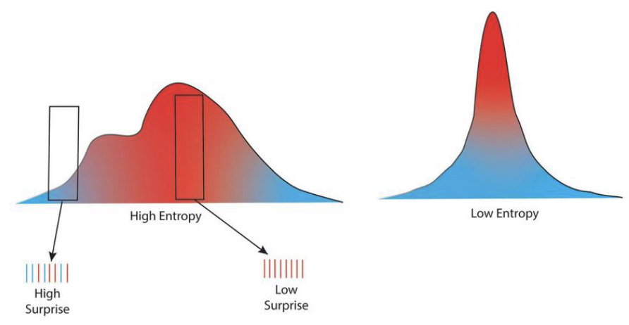
Left plot — High entropy: The distribution is broad/multimodal, so average unpredictability is high. A box over a blue, low-density region marks a high-surprise event; a box over a red, high-density region marks a low-surprise event.

Right plot — Low entropy: The distribution is sharply peaked; most mass sits near the center, so average unpredictability is low. Tail events would still be surprising, but they’re rare and contribute little to the average.

Cross-entropy¶

Cross-entropy between true $p$ and estimate $q$:

It is commonly used as a classification loss (negative log-likelihood).

KL divergence¶

KL divergence (not a metric):

asymmetric and violates triangle inequality. Minimizing $D_{\mathrm{KL}}(p\parallel q)$ fits $q$ to $p$.

Likelihood Function¶

Gaussian model and maximum likelihood¶

Assume $x_1,\dots,x_N$ are i.i.d. from $\mathcal{N}(\mu,\sigma^2)$.

• Likelihood and log-likelihood:

  $$\mathcal{L}(\mu,\sigma^2) = \prod_{n=1}^N \mathcal{N}(x_n\mid \mu,\sigma^2),\qquad \ell(\mu,\sigma^2)=\sum_{n=1}^N \log \mathcal{N}(x_n\mid \mu,\sigma^2).$$

  (10)

• Maximal Likelihood Estimate (MLE) (set derivatives to zero):

  $$\mu_{\text{ML}} = \frac{1}{N}\sum_{n=1}^N x_n,\qquad \sigma^2_{\text{ML}} = \frac{1}{N}\sum_{n=1}^N (x_n-\mu_{\text{ML}})^2.$$

  (11)

From single Gaussians to mixtures¶

A single Gaussian fails on multi-modal data. Increase flexibility with a mixture of $K$ Gaussians:

Direct MLE is hard because of the log-sum in $\ell(\theta)=\sum_n\log\sum_k \pi_k \mathcal{N}(x_n\mid\mu_k,\Sigma_k)$.

Latent variables and EM for GMMs¶

Introduce latent assignments $z_n\in\{1,\dots,K\}$ and work with responsibilities

Expectation–Maximization (EM) iterates:

• E-step: compute $\gamma_{nk}$ for all $n,k$ using current parameters.

• M-step: update parameters using soft counts $N_k=\sum_n \gamma_{nk}$:

  $$\mu_k \leftarrow \frac{1}{N_k}\sum_{n} \gamma_{nk} x_n,\quad \Sigma_k \leftarrow \frac{1}{N_k}\sum_{n} \gamma_{nk}(x_n-\mu_k)(x_n-\mu_k)^\top,\quad \pi_k \leftarrow \frac{N_k}{N}.$$

  (14)

  Each iteration does not decrease the data log-likelihood and converges to a local optimum.

Variational perspective and the ELBO¶

For latent-variable models, the marginal likelihood $\log p_\theta(x)=\log\int p_\theta(x,z)\,dz$ is intractable. Introduce a tractable $q_\phi(z\mid x)$ and use:

Thus $\mathcal{L}(\theta,\phi)\le \log p_\theta(x)$; maximizing the ELBO tightens the bound and implicitly makes $q_\phi$ approximate the true posterior.

Autoregressive density models (PixelRNN)¶

Use the chain rule to make likelihood tractable:

• Architecture idea: an RNN maintains a hidden state to summarize the context $x_{<i}$.

• Training: maximize log-likelihood (equivalently minimize cross-entropy). In practice use teacher forcing: feed the ground-truth prefix $x_{<i}$ when predicting $x_i$ to avoid error accumulation.

• Inference: sample sequentially from $p(x_i\mid x_{<i})$ (stochastic; slower than parallel decoders).

Pros

• Exact likelihood (good for model comparison),

• High-quality samples with sufficient capacity.

Cons

• Limited parallelism; slow sampling,

• Potential bias from raster order; capturing global context can be challenging.