Complex Processes

General Definitions¶

System Analysis & Modeling¶

System: An interconnected set of elements organized to achieve a specific function or purpose.

System Analysis: The science of studying systems to answer specific questions. Starting point is always the question. The question determines which parts of the system will be considered.

Model: A simplification of a real-world system used to answer specific questions. A model is a system itself that allows for experimentation (unlike the real system which might be too expensive, dangerous, or slow).

Simulation: The replication of a dynamic process in a model to achieve results transferable to reality.

Complex System: A system that evades simplification and remains multi-layered. To manage complexity, one should model specific problems or processes rather than the system as a whole.

Verification: Answering “Did we build the model right?” (Checking for bugs and logical consistency).

Validation: Answering “Did we build the right model?” (Checking if the model is suitable for the intended purpose and matches reality).

Decision Theory¶

Rational Decision: A decision process characterized by clear targets, objective information, and transparent rules or procedures.

Intuitive Decision: A decision based on experience and a “vast storehouse” of collective/unconscious knowledge rather than formalized procedures.

Mental Models: Internal conceptions that affect action (can be dangerous to base decisions on mental models). Scientific decision-making requires making these explicit and testing them against evidence (falsification).

Normative vs. Descriptive: Normative asks “What is the best decision?”; Descriptive asks “How do people actually decide?”.

Systems Thinking & Dynamics¶

Causal Loop Diagram (CLD): A qualitative diagramming tool used to visualize feedback structures. It uses variables and directed arrows with polarity to show causal links, without distinguishing between stocks and flows.

Reinforcing Loop (+): A feedback loop that amplifies change (contains an even number of negative signs).

Balancing Loop (-): A feedback loop that seeks stability or a goal (contains an odd number of negative signs).

Path Dependence: A dynamic behavior where small, random early events determine the final state, even if multiple end states were initially possible.

Lock-in: A situation where a system is stuck in a suboptimal equilibrium due to path-dependent processes.

System Analysis and Modeling¶

A system is a group of interacting entities defined by boundaries, structure, and purpose. System analysis is the science of studying these to answer specific questions. Modeling is an iterative process: Construct $\rightarrow$ Simplify $\rightarrow$ Model $\rightarrow$ Solve $\rightarrow$ Interpret $\rightarrow$ Validate $\rightarrow$ Present.

• White-box models: Based on theory and physical laws.

• Black-box models: Based on data pairs (AI/Machine Learning).

• Principle: “All models are wrong, but some are useful”—every model is a simplification.

Causal Models¶

3 Levels of formalisation:

Causal Loop Diagrams (CLD)¶

Communication-tool for causal structure in general discussion.

• Focus on feedback

• Focus on causality

• Caution: No focus on accumulation (see Stock-and-Flow Diagram for accumulation!

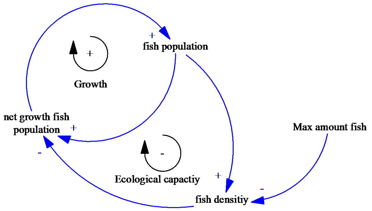
CLDs use variables and causal links with polarity marks to represent feedback structures.

• Polarity: A positive ($+$) mark means variables move in the same direction; a negative ($-$) mark means they move in opposite directions.

• Loops:

  • Reinforcing Loop ($+$): Amplifies change; has an even number of ($-$) signs.

  • Balancing Loop ($-$): Seeks stability/goals; has an odd number of ($-$) signs.

• Archetypes: Common patterns like “Fixes that Fail” (immediate fix with delayed negative reinforcement) or “Shifting the Burden” (symptomatic vs. fundamental solutions).

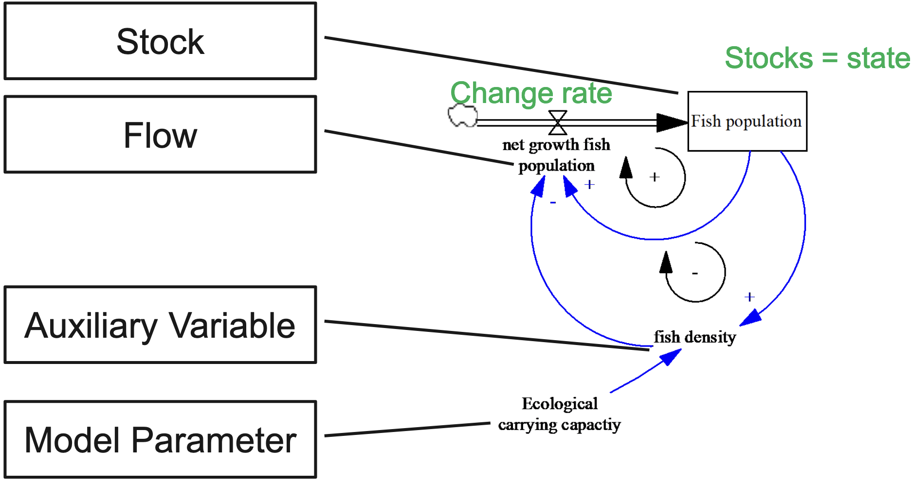
Stock-and-Flow Diagram¶

Precise visualization of Stocks and flows:

System Dynamics Simulation Model¶

Formal Simulation Model: Formulation of all Flows as equations, Enables quantitative simulation

Model assumptions:

• Continuous Time (Non-linear ordinary differential equation)

• Deterministic

• Homogeneity

• Perfect Mixing

• Emphasis on feedback, accumulation and delays

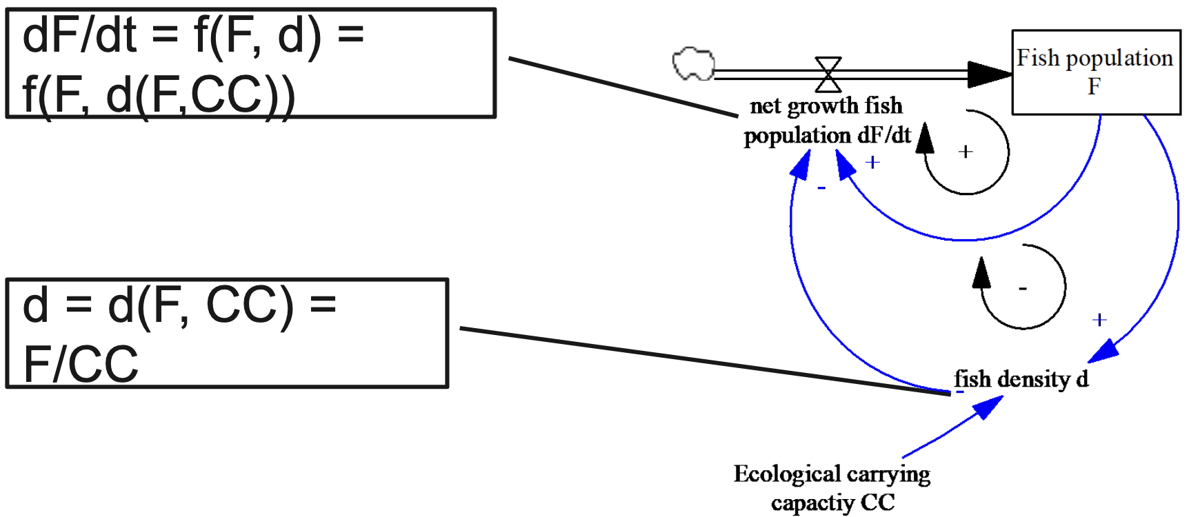
If you want to formulate a system dynamics simulation model model, you need to build a Stock-and-Flow Diagram first. Then add the auxilary variables and the parameters to the stocks and flows and then express all the flow variables and the auxiliary v variables as a function of their causes.

Path Dependence and Transitions¶

• Path Dependence: A process where small early events determine the final state.

  • Necessary Condition (not Sufficient Condition!) for Path Dependence: Reinforcing loops are required for path dependence to occur.

[Suppose] the evolution of a system is [deterministically] governed by its dynamic relations and its initial condition. Suppose the system converges for all or some set of initial conditions. There is path dependent if the limit depends on the initial conditions. - Definition according to Kenneth W. Arrow (2004)

Path dependence [is] a pattern of behavior in which small, random events early in the history of a system determine the end state, even when all end states are equally likely at the beginning. - Characterization according to Sterman (2000)

• Lock-in: A state where the system is stuck in a suboptimal equilibrium.

A process is locked-in to an outcome if, while at some point in history, minor influences could have caused the system to converge to another outcome, in the current situation, a relatively large effort is required to change it.

• Tipping Point: The boundary where a small change causes the system to shift to a different equilibrium.

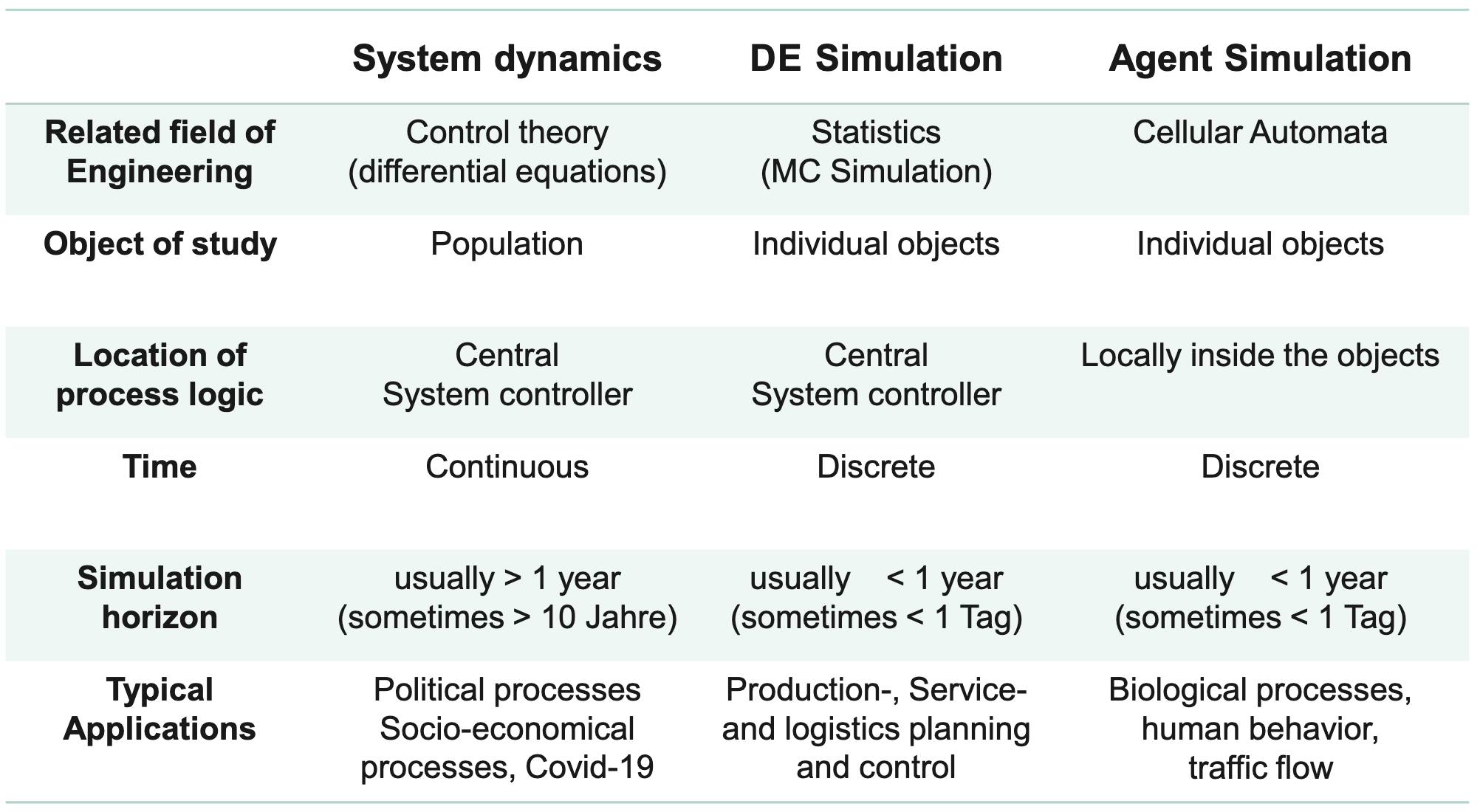
Simulation Paradigms¶

System Dynamics (SD): A method using stocks, flows, and feedback loops to model the behavior of populations or aggregates over continuous time.

Discrete Event Simulation (DES): A simulation paradigm where the system state changes only at discrete points in time (events). It tracks individual objects (items) flowing through servers and queues.

Agent-Based Simulation: A paradigm where a system consists of many individuals (agents) with simple internal logic/rules, whose interactions produce complex aggregate behavior.

Monte Carlo Simulation (MCS): A static simulation paradigm (no time dimension) that uses random sampling to approximate probabilities, areas, or averages.

Comparing Simulation Paradigms

Monte Carlo Simulation (MCS)¶

Monte Carlo Simulation is a numerical method for statistical calculation. It is based on using sequences of random numbers (resampling) in order to explore the behavior of the system. Monte Carlo Simulation exploits the computational power of computers.

In short: Its a static simulation paradigm using random sampling to calculate probabilities or averages.

MC can be considered a computer-science based alternative for classical (mathematics-based) statistics.

• Structure:

  1. Scenario Generator: Uses random generators (e.g., $X \sim U_c(min, max)$) to create $L$ scenarios.

  2. Calculation Scheme: Computes outcomes for each scenario.

  3. Aggregator: Summarizes results, usually as an average or probability.

• Formulas:

  • Probability: $P = \frac{\text{Successful Scenarios}}{L}$.

  • Expected Profit (News Vendor): $\text{Profit}_y = \min(N_y, Q) \times \text{Price} - Q \times \text{Cost}$.

  • Kinetic Energy: $E_{kin} = \sum_{y=1}^{L} \frac{1}{2} m_y (\omega r_y)^2$ where $m_y = \frac{M_{total}}{L}$.

Discrete Event Simulation (DES)¶

Tracks individual items (jobs) through servers at discrete points in time.

• Flow Blocks: Source, Sink, Queue, Server, Switch (picks one path), Junction (divergent = split; convergent = merge), and Gate (controls flow).

• Simulation Kernel: Manages a Future Event List (FEL) chronologically.

• Formulas:

  • Utilization ($U$): Fraction of time a server is busy.

    $$U = \text{Arrival Rate} (\lambda) \times \text{Avg. Processing Time} (\bar{s})$$

    (1)

    .

  • Multi-server Utilization: $U = \frac{\lambda \times \bar{s}}{c}$ where $c$ is the number of parallel servers.

  • Variation: Randomness (Coefficient of Variation) degrades performance more than high utilization.

Verification and Validation (V&V)¶

• Verification: “Did we build the model right?” (Checking for bugs).

  • Extreme Value Analysis: Testing “special” cases. Example: For $n=2$ random points on a circle ($r=1$), the average minimum distance is $\frac{\pi}{2}$.

  • Dimensional Analysis: Ensuring SI units match on both sides of a formula.

• Validation: “Did we build the right model?” (Checking if it suits the purpose).

  • Historical Data: Comparing simulated results to real-world performance.

  • Data Pitfall: Sales $\neq$ Demand (unsatisfied demand is hidden if stock is zero).

• Statistical Formula:

  • Confidence Interval Width: $\propto \frac{1}{\sqrt{n}}$ (to reduce interval width by 10, increase runs by 100).