ARIMA Models

Repetition¶

Autoregressive Models (AR)¶

We repeat the concept of autoregressive processes of order p (AR(p)-processes). Intuitively, the value of an AR(p) process at time $n$ is a linear combination of the $p$ previous values in the series. To be more precise

X_n = a_1 X_{n-1} + a_2 X_{n-2} + \dots + a_{n-p} X_{n-p} + W_n

(1)

$W_1, W_2, \dots$ is a white noise model with standard deviation $\sigma$ . We now will generate an AR(2) Model. Let us consider the AR(2) process

X_{n} =1.5 X_{n-1} - 0.9 X_{n-2} + W_n

(2)

from statsmodels.tsa.arima_process import ArmaProcess
import matplotlib.pyplot as plt
import numpy as np

ar2 = [1, -1.5, 0.9]
model = ArmaProcess(ar = ar2, ma = None)
simulated_data = model.generate_sample(nsample=1000)

plt.figure(figsize = (15,5))
plt.plot(simulated_data, '-')
plt.grid()
plt.title("AR(2)-Process")
plt.show()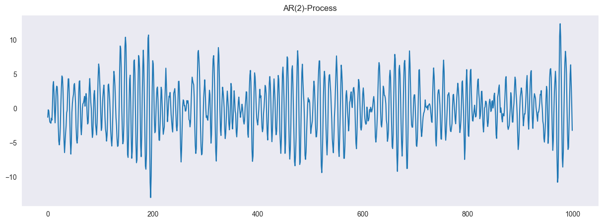

The characteristic polynomial is given by

\Phi(z) = 1 - a_1 z - a_2 z^2 - \dots - a_p z^p

(3)

If all roots of $\Phi(z)$ have an absolute value larger than 1, then the process is stationary. This can easily be checked with the model.isstationary command:

model.isstationary

True

We can even compute the complex roots of the polynomial, which are according to the lecture

z_{1,2} = \frac{5}{6} \pm \frac{i}{2}\sqrt{\frac{5}{3}}

(4)

model.arroots
np.abs(model.arroots)

array([1.05409255, 1.05409255])

Additionally, we compute the autocorrelation and partial autocorrelation both of the generated data (empirical autocorrelation function (acf) / partial autocorrelation function (pacf)) and for the process (theoretical). As we expect, the acf is oscillating and the pacf is vanishing after lags larger than $p$ .

from statsmodels.tsa.stattools import acf, pacf

fig, ax = plt.subplots(1,2, figsize = (15,5))
ax[0].plot(acf(simulated_data, nlags=40), label = "empirical acf")
ax[0].plot(model.acf(lags=40), label = "theoretical acf")
ax[0].legend()
ax[0].grid()

ax[1].plot(pacf(simulated_data, nlags=40), label = "empirical pacf")
ax[1].plot(model.pacf(lags=40), label = "theoretical pacf")
ax[1].legend()
ax[1].grid()

Moving Average Model (MA)¶

Moving average models can be used to model dependencies in the noise of a stochastic process. A moving average model of order $q$ (MA(q)-process) is defined as

X_n = W_n + b_1 W_{n-1} + \dots + b_q W_{n-q}

(5)

$W_1, W_2, \dots$ is a white noise model with standard deviation $\sigma$ . We now will generate an MA(4) Model. We consider the MA(4) process

X_n = W_n + 1.5 W_{n-1} + 1.1 W_{n-2} + W_{n-3} + 0.9 W_{n-4}

(6)

from statsmodels.tsa.arima_process import ArmaProcess
import matplotlib.pyplot as plt

ma4 = [1, 1.5, 1.1, 1, 0.9]
model = ArmaProcess(ar = None, ma = ma4)

simulated_data = model.generate_sample(nsample=500)

plt.figure(figsize = (15,5))
plt.plot(simulated_data, '-')
plt.grid()
plt.title("MA(5)-Process")
plt.show()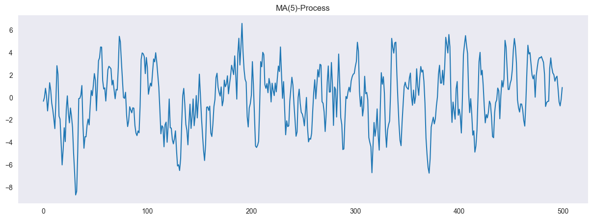

Moving average processes are always stationary but they are not unique in the sense that two different MA(q) processes can have the same autocorrelation function. Yet, there is always a unique process that is invertible. To check if a MA(q)-process is invertible we can investigate the roots of its characteristic polynomial

\Theta(z) = 1 + b_1 z + b_2 z^2 + \dots + b_q z^q

(7)

If all roots of $\Theta$ have absolute value larger than 1, then the process is invertible.

We check this for our process using the model.isinvertible command:

model.isinvertible

False

import numpy as np
np.abs(model.maroots)

array([0.92900679, 0.92900679, 1.13464461, 1.13464461])

We finally compute the autocorrelation and partial autocorrelation for our process (again, the empirical and the theoretical version). The acf of a MA(q) process vanishes for lags larger than $q$ and the pacf oscillates.

from statsmodels.tsa.stattools import acf, pacf

fig, ax = plt.subplots(1,2, figsize = (15,5))
ax[0].plot(acf(simulated_data, nlags=40), label = "empirical acf")
ax[0].plot(model.acf(lags=40), label = "theoretical acf")
ax[0].legend()
ax[0].grid()

ax[1].plot(pacf(simulated_data, nlags=40), label = "empirical pacf")
ax[1].plot(model.pacf(lags=40), label = "theoretical pacf")
ax[1].legend()
ax[1].grid()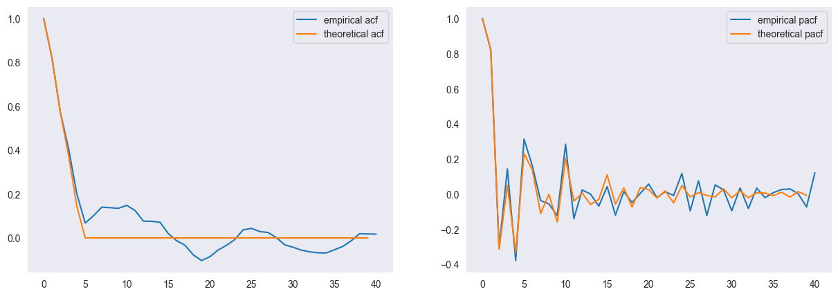

ARMA Model: AR and MA¶

By combining autoregressive and moving average models we arrive at ARMA(p,q)-processes. They are formally defined as

\Phi(B) X_n = \Theta(B) W_n

(8)

where $\Phi$ and $\Theta$ are the characteristic polynomials of the autoregressive and moving average model respectively and $B$ is the backshift operator, i.e.

B(X_n) = X_{n-1}

(9)

In particular, we have

\Phi(B) X_n = X_n - a_1 X_{n-1} - \dots - a_{p} X_{n-p}

(10)

and

\Theta(B) W_n = W_n - b_1 W_{n-1} - \dots - b_{q} X_{n-q}

(11)

In the following, we will generate an AR(2,2) process. We define the ARMA(2,2) process as

We define the ARMA(2,2) process as

X_n = 1.5 X_{n-1} - 0.9 X_{n-2} + W_n + 1.5 W_{n-1} + 2.2 W_{n-2}

(12)

(1 - 1.5 B + 0.9 B^2) X_n = (1 + 1.5 B + 2.2 B^2) W_n.

(13)

from statsmodels.tsa.arima_process import ArmaProcess
import matplotlib.pyplot as plt

ar2 = [1, -1.5, 0.9]
ma2 = [1, 1.5, 2.2]
model = ArmaProcess(ar = ar2, ma = ma2)
simulated_data = model.generate_sample(nsample=300)

plt.figure(figsize = (15,5))
plt.plot(simulated_data, '-')
plt.title("ARMA(2,2)-process")
plt.grid()
plt.show()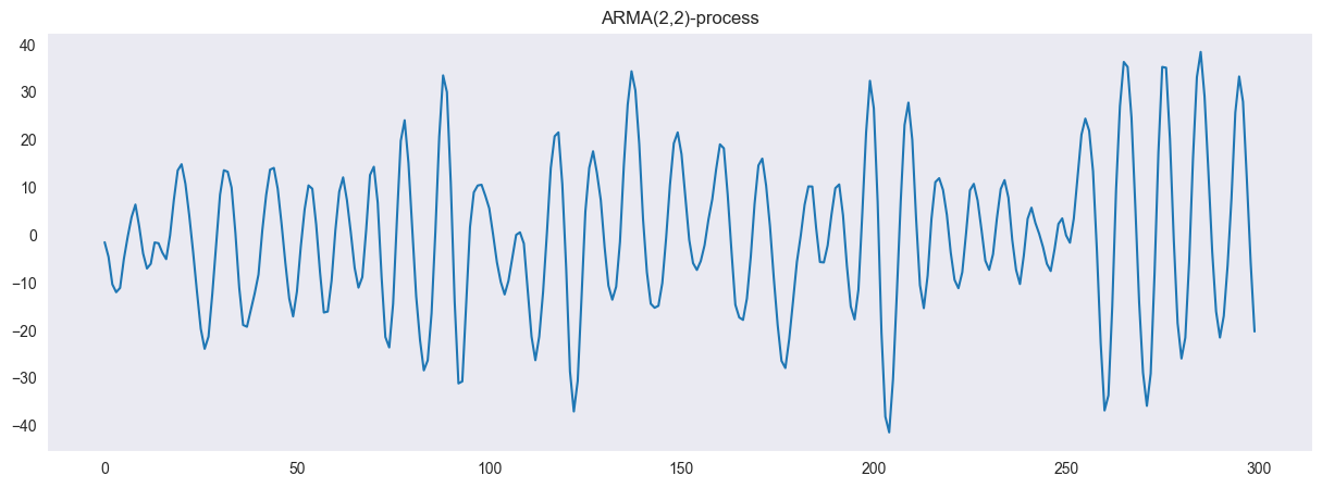

We can check the stationarity and causality of the model as with the pure AR(p) and MA(q) processes, i.w. via the roots of the repsective characteristic polynomials.

import numpy as np

print(model.isstationary)
print(np.abs(model.arroots))

True
[1.05409255 1.05409255]

import numpy as np

print(model.isinvertible)
print(np.abs(model.maroots))

False
[0.67419986 0.67419986]

The acf and pacf for an ARMA(p,q) model do not have any distinct cut-off behaviour that aids for model selection. We demonstrate this with the simulated data.

from statsmodels.tsa.stattools import acf, pacf

fig, ax = plt.subplots(1,2, figsize = (15,5))
ax[0].plot(acf(simulated_data, nlags=40), label = "Empirical acf")
ax[0].plot(model.acf(lags=40), label = "Theoretical acf")
ax[0].legend()
ax[0].grid()

ax[1].plot(pacf(simulated_data, nlags=40), label = "Empirical pacf")
ax[1].plot(model.pacf(lags=40), label = "Theoretical pacf")
ax[1].legend()
ax[1].grid()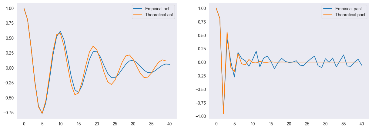

Estimating ARMA(p,q) from data¶

We are now given a time series $x_1, x_2, \dots$ and we want to estimate for a given order $(p,q)$ the coefficients $a_1, \dots, a_p$ and $b_1, \dots, b_q$ . We showed the maximum likelihood method as one approach (although there are different ways to estimate the coefficients)

from statsmodels.tsa.arima.model import ARIMA
import matplotlib.pyplot as plt
import pandas as pd
import numpy as np

df = pd.read_csv("data/TeslaIdx1.csv", sep ="\t")
df.head()

We turn the data frame into a times series object

df['Date'] = pd.to_datetime(df['Date'])
df.set_index('Date', drop = True, inplace=True)
df.head()

---------------------------------------------------------------------------
KeyError                                  Traceback (most recent call last)
File ~/Development/marbetschar/notes/.venv/lib/python3.12/site-packages/pandas/core/indexes/base.py:3812, in Index.get_loc(self, key)
   3811 try:
-> 3812     return self._engine.get_loc(casted_key)
   3813 except KeyError as err:

File pandas/_libs/index.pyx:167, in pandas._libs.index.IndexEngine.get_loc()

File pandas/_libs/index.pyx:196, in pandas._libs.index.IndexEngine.get_loc()

File pandas/_libs/hashtable_class_helper.pxi:7088, in pandas._libs.hashtable.PyObjectHashTable.get_item()

File pandas/_libs/hashtable_class_helper.pxi:7096, in pandas._libs.hashtable.PyObjectHashTable.get_item()

KeyError: 'Date'

The above exception was the direct cause of the following exception:

KeyError                                  Traceback (most recent call last)
Cell In[4], line 1
----> 1 df['Date'] = pd.to_datetime(df['Date'])
      2 df.set_index('Date', drop = True, inplace=True)
      3 df.head()

File ~/Development/marbetschar/notes/.venv/lib/python3.12/site-packages/pandas/core/frame.py:4113, in DataFrame.__getitem__(self, key)
   4111 if self.columns.nlevels > 1:
   4112     return self._getitem_multilevel(key)
-> 4113 indexer = self.columns.get_loc(key)
   4114 if is_integer(indexer):
   4115     indexer = [indexer]

File ~/Development/marbetschar/notes/.venv/lib/python3.12/site-packages/pandas/core/indexes/base.py:3819, in Index.get_loc(self, key)
   3814     if isinstance(casted_key, slice) or (
   3815         isinstance(casted_key, abc.Iterable)
   3816         and any(isinstance(x, slice) for x in casted_key)
   3817     ):
   3818         raise InvalidIndexError(key)
-> 3819     raise KeyError(key) from err
   3820 except TypeError:
   3821     # If we have a listlike key, _check_indexing_error will raise
   3822     #  InvalidIndexError. Otherwise we fall through and re-raise
   3823     #  the TypeError.
   3824     self._check_indexing_error(key)

KeyError: 'Date'

We compute the log-returns of the stock index for the closing value of the index, i.e.

r^\text{log}_n = \log\left(\frac{X_{n}}{X_{n-1}}\right)

(14)

lr = np.log(df.Close.values[1:]/df.Close.values[:-1])
lr = np.r_[np.NaN, lr]
df['LogRet'] = lr
df['LogRet'].plot(figsize = (15,5))
plt.grid()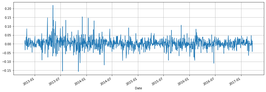

We use the ARIMA class to estimate the parameters. To this end, we initialize the class with the observed series and the order of the model. By calling .fit() the model parameters are estimated. The summary function gives a comprehensive report on the model.

df.dropna(axis = 0, inplace = True)
model = ARIMA(df.LogRet, order = (1,0,1))
res = model.fit()
print(res.summary())

                               SARIMAX Results                                
==============================================================================
Dep. Variable:                 LogRet   No. Observations:                 1111
Model:                 ARIMA(1, 0, 1)   Log Likelihood                2308.225
Date:                Wed, 13 Dec 2023   AIC                          -4608.449
Time:                        13:20:25   BIC                          -4588.397
Sample:                             0   HQIC                         -4600.867
                               - 1111                                         
Covariance Type:                  opg                                         
==============================================================================
                 coef    std err          z      P>|z|      [0.025      0.975]
------------------------------------------------------------------------------
const          0.0020      0.001      2.111      0.035       0.000       0.004
ar.L1         -0.2060      0.864     -0.238      0.812      -1.899       1.487
ma.L1          0.2277      0.864      0.263      0.792      -1.467       1.922
sigma2         0.0009   2.01e-05     45.762      0.000       0.001       0.001
===================================================================================
Ljung-Box (L1) (Q):                   0.00   Jarque-Bera (JB):              1953.04
Prob(Q):                              0.99   Prob(JB):                         0.00
Heteroskedasticity (H):               0.39   Skew:                             0.49
Prob(H) (two-sided):                  0.00   Kurtosis:                         9.42
===================================================================================

Warnings:
[1] Covariance matrix calculated using the outer product of gradients (complex-step).

The summary shows that the estimated coefficients are not significantly different from 0 which means, that the time series can not be modelled by means of an AR(1,1) model. This is also the reason why you whitness different coefficients compared to the slides: Since there is no real model describing the log-returns of the Tesla stock index the estimated coefficients are just due to some numerical algorithm. Depending on the algorithm implementation you will receive other results.

The plot below showing the predicted values further stresses the fact that modelling of the log-returns is futile.

plt.figure(figsize = (15,5))
plt.plot(res.predict())
df.LogRet.plot()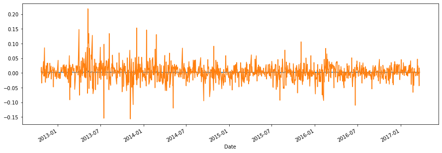

Model selection for ARMA(p,q)¶

So far we did not bother about choosing the model order. However, this is a delicate task since the acf and pacf plots no longer help in this respect. Instead we will focus on the Akaike information criterion (AIC) as a goodness-of-fit measure that is comparable across various model dimensions. It is defined as

AIC(p,q) = -2\cdot \log(L(\vec \theta, \vec x )) + 2(p + q + 1)

(15)

Here $L$ is the likelihood function of the problem and $\vec\theta$ the vector of all unknown parameters in the model. The vector $\vec x$ contains the time series data that we want to model. For a fitted model - let us choose arbitrarily the model ARIMA(2,1,2) - the AIC value can be retrieved.

from statsmodels.tsa.arima.model import ARIMA
import matplotlib.pyplot as plt
import pandas as pd
import numpy as np
import warnings
warnings.filterwarnings("ignore")

df = pd.read_csv("data/temperatures.csv")
df['Year'] = pd.to_datetime(df['Year'], format="%Y")
df.set_index('Year', drop = True, inplace=True)
df.dropna(axis = 0, inplace = True)
model = ARIMA(df.Value, order = (2,1,2))
res = model.fit()
print(res.aic)

125.28563917508072

The model predictions look as follows:

# Plot the original data

temp = df['Value']
plt.figure(figsize=(10, 6))
plt.plot(temp, label='Data', color='black', linewidth=2)
plt.plot(temp - res.resid, label='ARIMA(2,1,2) model', color='red', linewidth=2)
plt.title("Global Temperature Differences")
plt.ylabel("Temperature Difference")
plt.legend()
plt.show()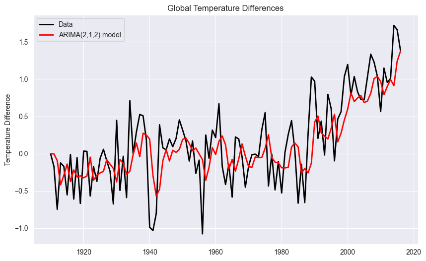

How do we determine the differencing order $d$ and the order parameters $p$ for the AR(p) process and $q$ for the MA(q) process?

STEP 1 : Determine the Differencing Order d¶

We start with order $d=1$ , i.e., we compute the differences of the temperatures

Y_n = X_{n} - X_{n-1} = (1 - B) X_n

(16)

# Extract the temperature column
temp = df['Value']

# Plot the first order difference
plt.figure(figsize=(10, 6))
plt.plot(temp.diff(), label='Yearly Difference', color='blue', linewidth=2)
plt.title("Yearly Difference for Temperature")
plt.ylabel("Difference")
plt.grid(True)
plt.show()

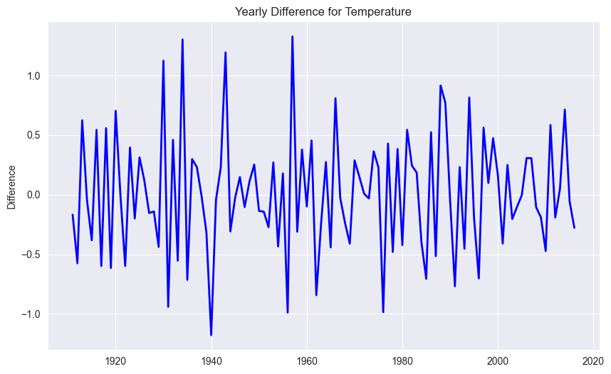
The trend is not any more visible. Thus, we choose $d=1$ as differencing order.

STEP 2 : Determine the Order Parameters p and q¶

We now simply loop over a range of candidate model and select the best model in terms of the lowest AIC value. This is a brute force method that is limited by the amount of candidate model that we consider.

from itertools import product
import seaborn as sns
import warnings
warnings.filterwarnings("ignore")

ar = np.arange(8)
ma = np.arange(8)

AIC = np.zeros((8,8))
for comb in product(ar, ma):
    p = comb[0]
    q = comb[1]
    model = ARIMA(temp, order = (p,1,q))
    res = model.fit()
    AIC[p,q] = res.aic

plt.figure(figsize=(8, 6))
ax = sns.heatmap(AIC, cmap='coolwarm')

# Labeling
ax.set_xlabel('p')
ax.set_ylabel('q')
ax.set_title('Heatmap with different order parameters p and q ')
plt.show()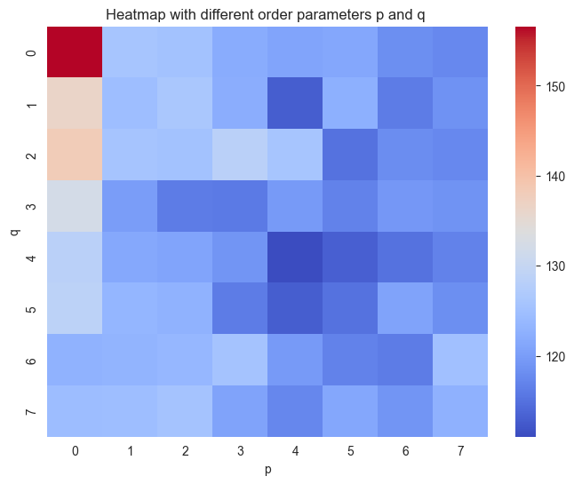

On the basis of the heatmap, we choose $p=4$ and $q=4$ which shows the lowest AIC value.

import numpy as np
import matplotlib.pyplot as plt
from statsmodels.tsa.arima.model import ARIMA

# Fit the ARIMA model
model_opt = ARIMA(temp["1910":"2006"], order=(4, 1, 4)).fit()

# Predict including confidence interval
pred = model_opt.get_prediction(start="2007", end="2016")
pred = pred.prediction_results
pred_cov = pred._forecasts_error_cov
pred = pred._forecasts[0]
pred_upper = pred + 1.96 * np.sqrt(pred_cov[0][0])
pred_lower = pred - 1.96 * np.sqrt(pred_cov[0][0])

# Plot
x = temp.index.year
x_pred = np.arange(2006, 2016)
fig = plt.figure(figsize=(10, 5))
ax = fig.add_subplot(1, 1, 1)
ax.plot(x[:97], temp["1910":"2006"], '-k', label='train data')
ax.plot(x[96:], temp["2006":"2016"], 'b', label='validation data')
ax.plot(x_pred, pred, 'r', label='Prediction')
ax.plot(x_pred, pred_upper, ':b', label='95% conf')
ax.plot(x_pred, pred_lower, ':b')
ax.plot([x[0], x_pred[-1]], [0, 0], ':k')
plt.xlabel("Time")
plt.ylabel("Values")
plt.legend()
plt.show()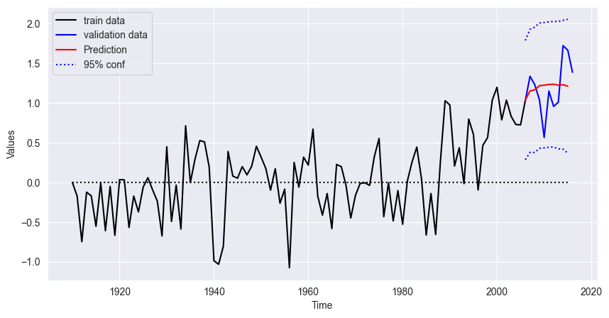

Performance Metrics¶

MAE¶

# Actual values for the prediction period
observed_values = temp["2007":"2016"]
pred = model_opt.get_prediction(start="2007", end="2016")
pred = pred.prediction_results
predicted_values = pred._forecasts[0]

# Calculating MAE
mae = np.mean(np.abs(predicted_values - observed_values))
print("Mean Absolute Error (MAE):", mae)

Mean Absolute Error (MAE): 0.28410908386305544

RMSE¶

# Calculating RMSE
rmse = np.sqrt(np.mean((predicted_values - observed_values) ** 2))
print("Root Mean Square Error (RMSE):", rmse)

Root Mean Square Error (RMSE): 0.3373007497235178

MAPE¶

# Calculating MAPE
mape = np.mean(np.abs((observed_values - predicted_values) / observed_values)) * 100
print("Mean Absolute Percentage Error (MAPE):", mape, "%")

Mean Absolute Percentage Error (MAPE): 28.186547936354867 %

Quartile Score¶

import scipy.stats as stats

# Forecast
forecast_length = len(predicted_values)
forecast_result = model_opt.get_forecast(steps=forecast_length)
forecast_mean = forecast_result.predicted_mean
forecast_std = np.sqrt(forecast_result.var_pred_mean)

# Function to compute quantile forecasts
def compute_quantile_forecasts(mean, std, quantiles):
    forecasts = {}
    for quantile in quantiles:
        z_score = stats.norm.ppf(quantile)
        forecasts[quantile] = mean + z_score * std
    return forecasts

# Quantiles to compute
quantiles = [0.25, 0.5, 0.75]

# Compute quantile forecasts
quantile_forecasts = compute_quantile_forecasts(forecast_mean, forecast_std, quantiles)

# Function to calculate pinball loss
def pinball_loss(y_true, y_pred, quantile):
    delta = y_true - y_pred
    return np.mean(np.where(delta >= 0, quantile * delta, (quantile - 1) * delta))

# Calculate quartile scores for each quantile forecast
quartile_scores = {}
for quantile in quantiles:
    quartile_scores[quantile] = pinball_loss(observed_values, quantile_forecasts[quantile], quantile)

# Display the quartile scores
for quantile, score in quartile_scores.items():
    print(f"Quartile score for quantile {quantile}: {score}")

Quartile score for quantile 0.25: 0.10999166116844598
Quartile score for quantile 0.5: 0.14205454193152772
Quartile score for quantile 0.75: 0.1068138721138264

SARIMA Model¶

import numpy as np
import pandas as pd
import matplotlib.pyplot as plt

# loading data
AirP = pd.read_csv('data/AirPassengers.csv')

# creating pandas DateTimeIndex
dtindex = pd.DatetimeIndex(data = pd.to_datetime(AirP['TravelDate']), freq = 'infer')

# setting as Index
AirP.set_index(dtindex, inplace = True)
AirP.drop('TravelDate', axis = 1, inplace = True)

# plotting data
plt.plot(AirP)
plt.xlabel('time')
plt.ylabel('Passengers in 1000')
plt.grid()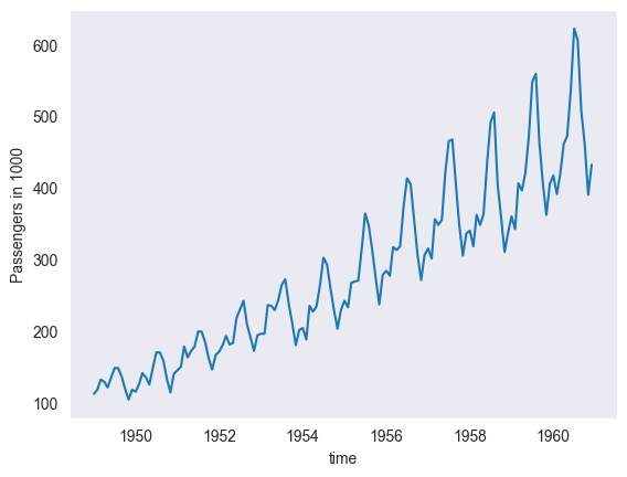

# STEP: transforming the data (for stationarity)

# --- there is an increasing variance -> let's "stabilize" the variance by transforming the data
# (with Box-Cox transform with lambda = 0, therefore just taking the log)
AirP_TRA = np.log(AirP['Passengers']) # TRA <-> transformed

# plotting
plt.plot(AirP_TRA)
plt.xlabel('time')
plt.ylabel('ln(Passengers)')
plt.title('Box-Cox transform: lambda = 0')
plt.grid()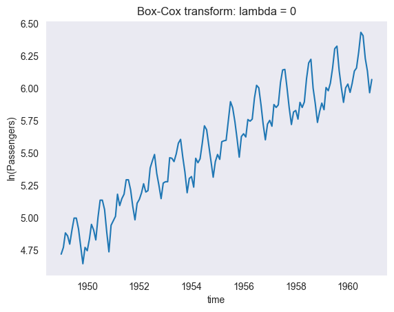

# --- there is a trend -> let's apply "differencing" to AirP_TRA
AirP_TRA_1 = AirP_TRA.diff()

# plotting
plt.plot(AirP_TRA_1)
plt.xlabel('time')
plt.ylabel('ln(Passengers)')
plt.title('Differencing: d = 1')
plt.grid()

# OK for d = 1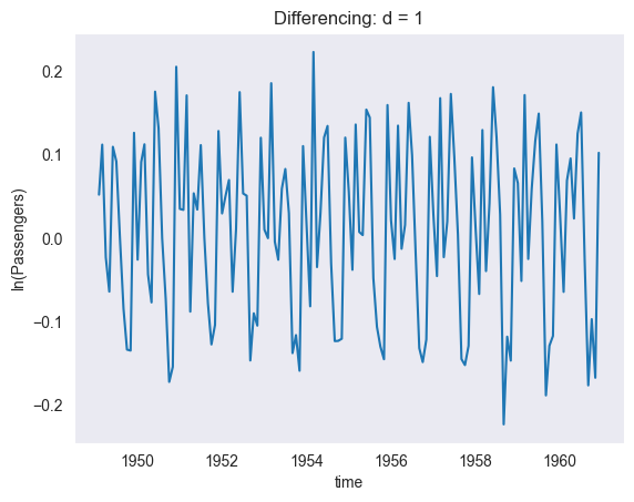

# --- there is seems to be a seasonality -> let's apply "differencing" for lag 12 to AirP_TRA_1
AirP_TRA_1_12 = AirP_TRA_1.diff(periods = 12)

# plotting
plt.plot(AirP_TRA_1_12)
plt.xlabel('time')
plt.ylabel('ln(Passengers)')
plt.title('Differencing: s = 12')
plt.grid()

# OK for s = 12

# STEP: determining the values of "order" parameters P and Q (seasonal)

# plotting the empirical autocorrelation (acf) and empirical partial autocorrelation (pacf)
from statsmodels.graphics.tsaplots import plot_acf, plot_pacf

fig = plt.figure(figsize = (14, 5))
ax1 = fig.add_subplot(1, 2, 1)
plot_acf(AirP_TRA_1_12.dropna(), lags = 50, ax = ax1, title = 'Empirical Autocorrelation')
ax1.plot([12, 12], [-1, 1], ':r')
ax2 = fig.add_subplot(1, 2, 2)
plot_pacf(AirP_TRA_1_12.dropna(), lags = 50, ax = ax2, title = 'Empirical Partial Autocorrelation')
ax2.plot([12, 12], [-1, 1], ':r')

# OK for P = 1 and Q = 1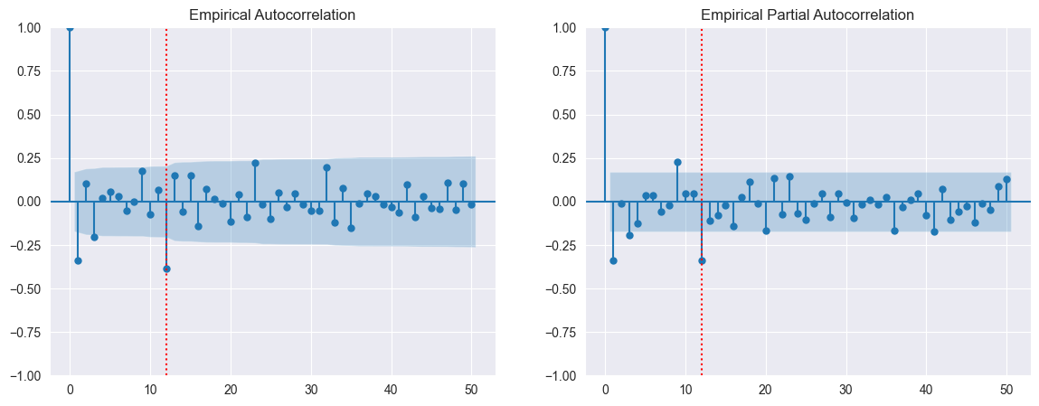

# STEP: determine the values of "order" parameters p and q (non-seasonal)

from statsmodels.tsa.arima.model import ARIMA
from itertools import product
import seaborn as sns

p = np.arange(4)
q = np.arange(5)

AIC = np.zeros((len(p), len(q)))
for comb in product(p, q):
    p_ind = comb[0]
    q_ind = comb[1]
    model = ARIMA(AirP_TRA, order = (p_ind, 1, q_ind), seasonal_order = (1, 1, 1, 12))
    res = model.fit()
    AIC[p_ind, q_ind] = res.aic


# plotting heatmap
plt.figure(figsize = (8, 6))
ax = sns.heatmap(AIC, cmap = 'coolwarm')
ax.set_xlabel('q')
ax.set_ylabel('p')
ax.set_title('Heatmap with different order parameters p and q ')
plt.show()

# OK for p = 0 and q = 1
result = ARIMA(AirP_TRA, order = (0, 1, 1), seasonal_order = (1, 1, 1, 12)).fit()
result.aic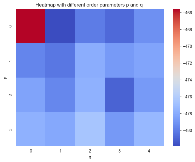

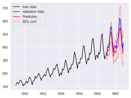
-481.9060733749852

# STEP: forecasting

from statsmodels.tsa.arima.model import ARIMA

# fitting SARIMA model on data from 1949-01 to 1958-12
model_opt = ARIMA(AirP_TRA['1949':'1958'], order = (0, 1, 1), seasonal_order = (1, 1, 1, 12)).fit()

# computing predictions (including confidence interval)
pred = model_opt.get_prediction(start = '1959-01-01', end = '1960-12-01')
pred = pred.prediction_results
pred_cov = pred._forecasts_error_cov
pred = pred._forecasts[0]
pred_upper = pred + 1.96 * np.sqrt(pred_cov[0][0])
pred_lower = pred - 1.96 * np.sqrt(pred_cov[0][0])

# plotting results in original variables (i.e. after inverse Box-Cox)
# time interval for prediction
t_pred = AirP_TRA['1959':'1960'].index
plt.plot(AirP['1949':'1958'], '-k', label = 'train data')
plt.plot(AirP['1959':'1960'], 'b', label = 'validation data')
plt.plot(t_pred, np.exp(pred), 'r', label = 'Prediction')
plt.plot(t_pred, np.exp(pred_upper), ':r', label = '95% conf')
plt.plot(t_pred, np.exp(pred_lower), ':r')
plt.legend()
plt.show()